The Shape of a Photon

Multi-dimensional Space

Imaginary numbers are invaluable in many areas of mathematics, physics, and engineering. But in general, they are abstract entities with no real world analog. This, however, is not true, when we enter into the strange world of Quantum Mechanics, where imaginary numbers take on a real and — in some sense — measurable significance.

Recent developments in our understanding of imaginary numbers has led people to equate the Real number system with the XOR logic gate and the Imaginary number system with XNOR.[] []

In quantum mechanics, imaginary numbers are used to explain and represent the fact that a particle’s momentum and position are two different and interlinked properties of the particle.

In this most simple example of a plane wave, we see the variable ‘i’ as an exponent value.[] The presence of ‘i’ in equations such as these has a very severe consequence, as knowing the momentum of a particle exactly, results in its position being everywhere at once and vice versa. To avoid running into these infinities, we can only ever know these two properties of the wave function approximately. This level of uncertainty is a consequence of the Schrödinger Equation and the Heisenberg Uncertainty Principle.

To demonstrate this bizarre relationship between momentum and position, the imaginary part of the wave function must be raised to its power. This cancels out the imaginary part of the equation to give us the absolute value. A similar result can be achieved with XNOR (!∆) and XOR (∆). This is because XOR and XNOR are non-commutative, !∆.∆ + ∆.!∆ = 0, just like the Quaternions and Octonions. By privileging the XNOR value, we can obtain the real absolute value for Complex number. The equation must be run twice; once for XNOR and then for XOR, and the results of both equations are summed together. Using a simple polynomial example, we get;

(x!∆+y∆)(x!∆+y∆)

a: -x!∆2 - 2x!∆y∆ - y∆

b: x!∆2 + 2x!∆y∆ + y∆

a + b = 0

Using this polynomial equation we can graph various surfaces in both XOR and XNOR space. Our XOR universe has three spatial dimensions. The fourth spatial dimension is the XNOR imaginary axis. If we want the exact position of our particle, we need to give it a real numbered value in each of our 3 XOR axes. When these three axes are combined with the fourth imaginary axis, they cancel each other out. This cancellation results in the flat plane that denotes the particle being in all positions or momentums at once. Plotting the above example in dimensions ‘∆, ∆, !∆’, gives this result:

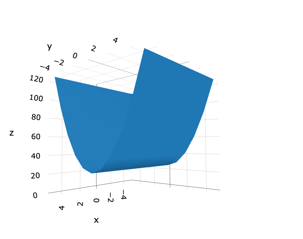
Figure 1: Quadratic curve (∆z+∆y+!∆x)3

Where as plotting ‘∆, ∆, ∆, !∆’, which is a fourth-dimensional coordinate results in the flat plane:

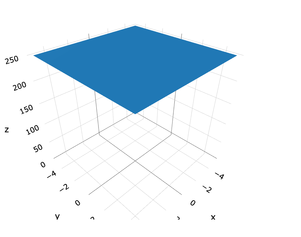
Figure: (∆w+∆z+∆y+!∆x)3

This achieves the same results as the complex quantum mechanical equation with a minimum of the effort, in fact anyone with even basic algebra skills could do these calculations by hand, on a sheet of paper. I refer to these different number systems as Dimensional Gate Operators (DGO), because they express dimensionality through operators based on logic gates.

A Better Example

When graphing the position or momentum of a particle, it is more accurate to use waveforms than mere polynomials. This waveform represents the exact momentum of a particle at time t.

Once again, applying the XNOR and XOR gates to this we get the position value for this wave function;

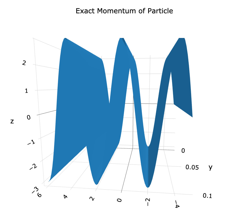
Figure 3: Cos(∆x)

Since we are able to graph the XOR momentum-space component, it is a trivial matter to calculate the XNOR position-space component, which will simply be its inverse, in this simple scenario.

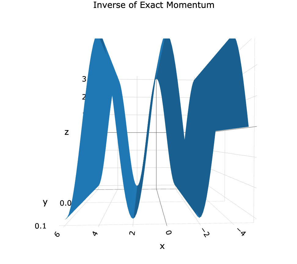
Figure 4: Cos(!∆x)

Now that we have both wave functions existing in separate spaces, we can graph them together. This is something which is ordinarily forbidden in quantum mechanics.

Figure 5: Exact momentum and position-state superimposed

From this perspective, it becomes apparent why the Heisenberg Uncertainty Principle exists. The two wave functions cancel out and what is left is the infinite value plane in the fourth dimension, which is truly infinite. This cancellation is similar to orthogonality in linear algebra, which suggests that this is how particles actually look, when viewed from both sides of the XOR and XNOR axes simultaneously.

Figure 6

A More Complex Example

So far, we have been using a plane sine wave to describe fundamental particles. It is clear that if we are to get a better understanding, we will have to progress to a more accurate model of the photon. For this, I have chosen initially the Mexican Hat function:

This produces a graph, which looks like this in XOR:

Figure 7: Mexican Hat Graph

For practical reasons this model is too simple, as it does not include the discrete nature of a pattern that we would expect to see. We will remedy this in the next section. For now lets take a look at how our graph looks in XNOR:

Figure 8

Notice how this ‘wave function’ — although it no longer looks like a wave — curves downwards at the bottom. This is suggestive of hyper-dimensionality that I have observed in other higher-dimensional algebraic graphs and suggests that this is truly a 3-D representation of something that is actually 4-dimensional.

We also see a series of strange lines.

What these represent is the points at which the square roots of the x2 and y2 components equal zero. These points go to infinity or are otherwise undefined. Their cross shape is the result of the traces of the matrix division/multiplication (depending on the function that you use). I chose a value of ‘1’ to replace the infinities, but as we know any real value integer could serve the same purpose. Adding in a value of -1 produces an entirely different result, which we will look at and examine later.

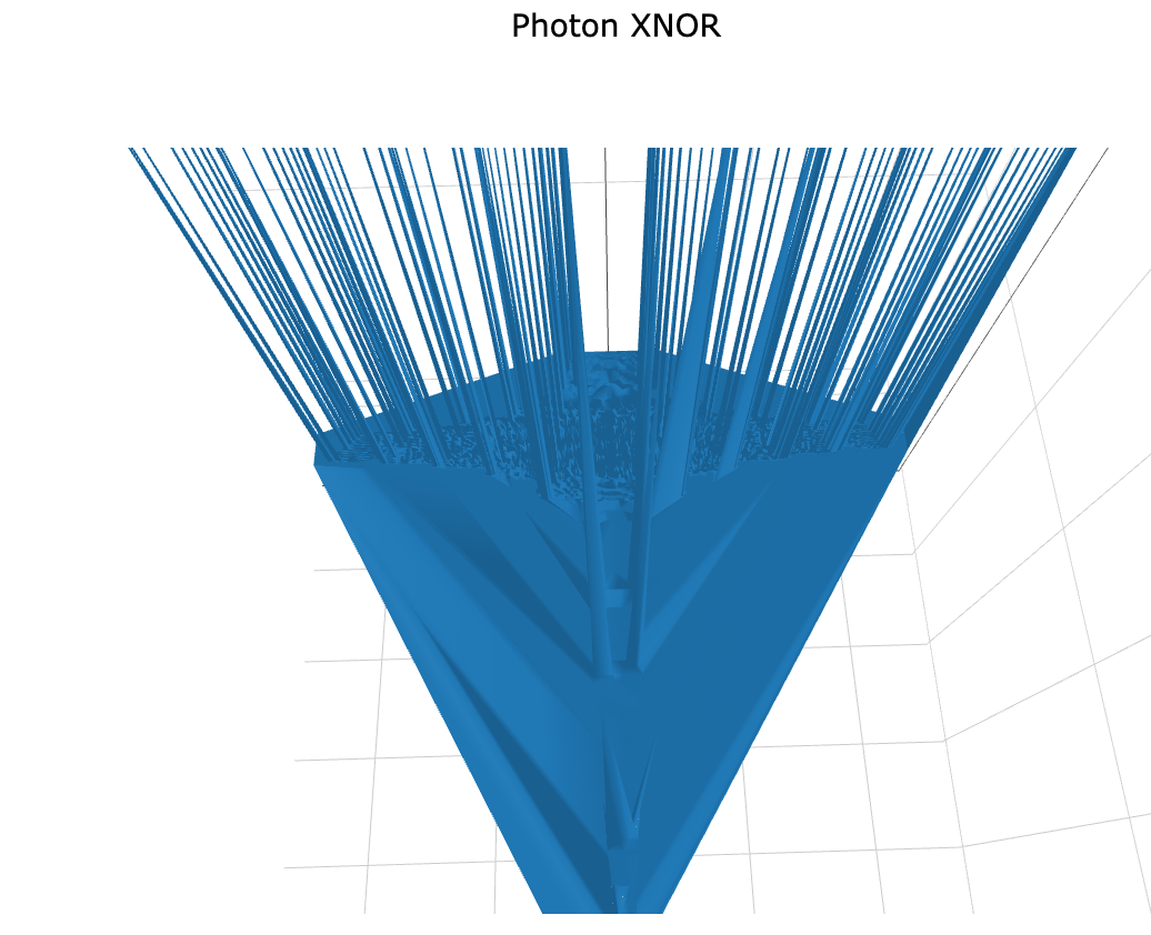
Figure 9

Another way to view this data is to set the results of our XOR calculation as our y-axis and the results of our XNOR calculation, as our z-axis. This means that the two separate results of the XOR and XNOR calculation become a new coordinate set, which obviously has its advantages, when visualising 4-dimensional space.

What we see here is that the waveform completely cancels out in 4D space, leaving only the infinite values. This tells us that the Mexican Hat diagram is not a valid waveform for the photon. We will need something a little more complex…

An Even More Complex Example

Asides for some complications with the exponential function, Sin and Cos, which need to be properly accounted for, the mathematics in XNOR and its confluence with XOR is relatively straightforward. Using the function for a discrete wave packet in a 3D XOR state, we have:

When we plot this we get the following:

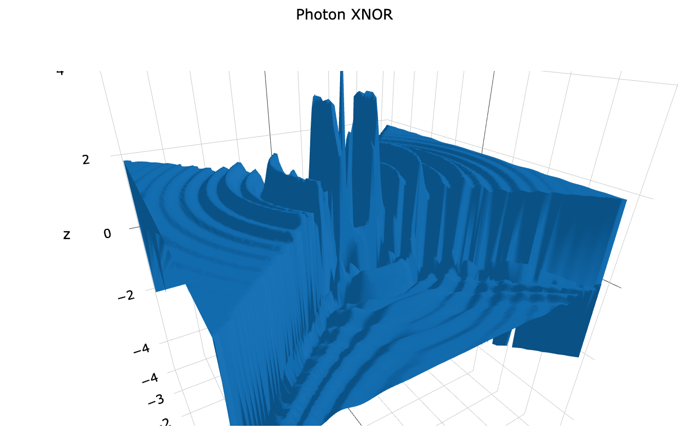
Figure 10

Again, we see this cross-shape, where the x2 and y2 components equal zero and are therefore infinite. Before, I replaced this value with ‘1’, for convenience, but now I’m going to use ‘-1’, which is much more in keeping with XNOR. A value of -0.8 works even better. When we do this, it flattens the graph down, which is a much more reasonable result;

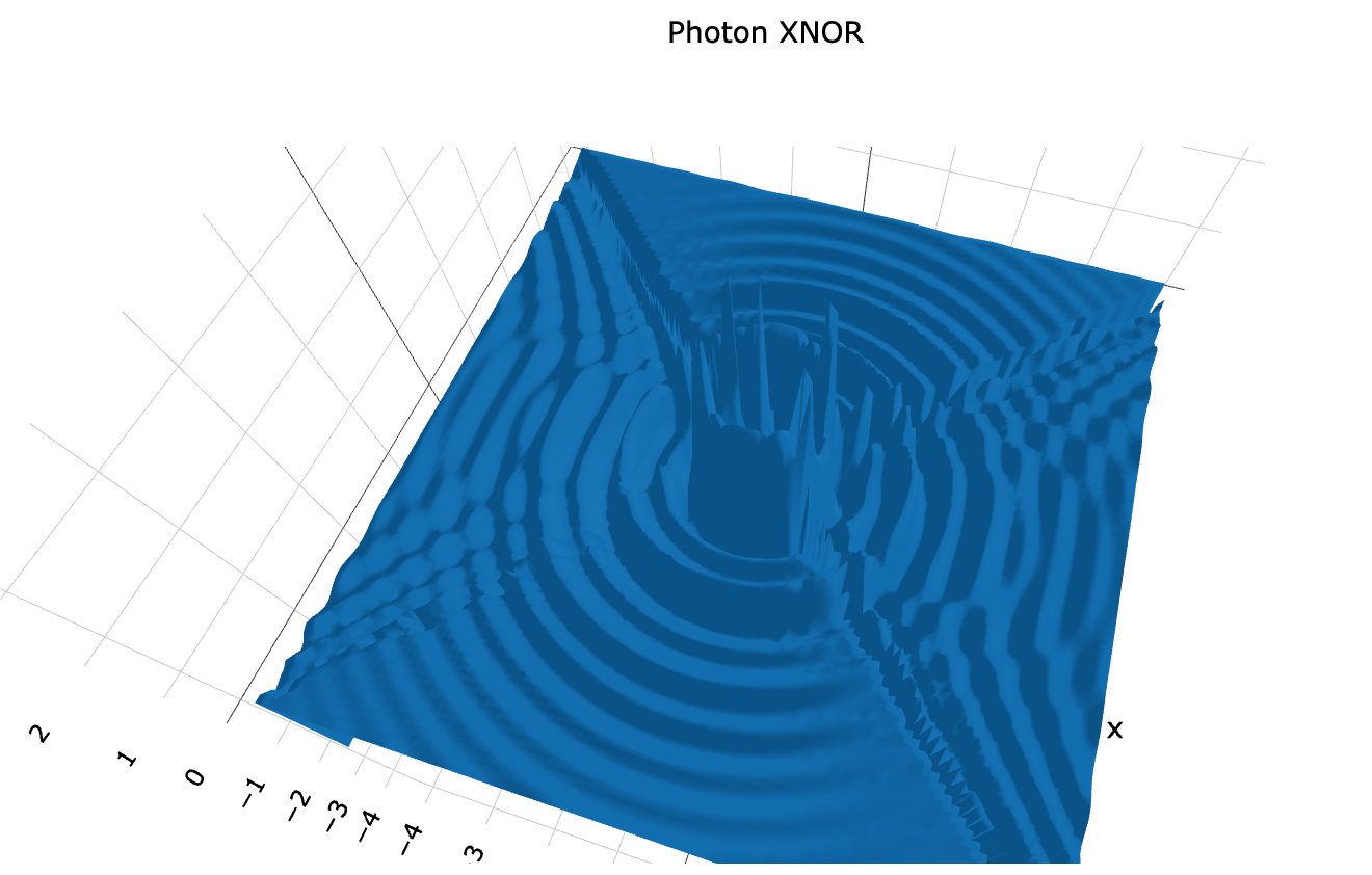
Figure 11

Interestingly, this XNOR wave function for the photon looks very similar to the theoretical predictions based on the Schrödinger equation (below right), as well as experimental imaging evidence carried out by physicists at the University of Warsaw (below left).[]

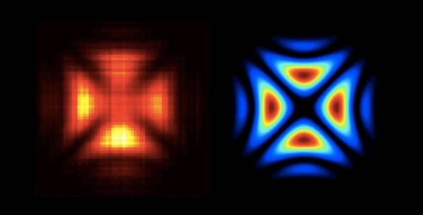
Figure 12

Graphing this purely in XNOR we get this result:

Figure 13

With this more complex example, we see that only half of the wave function cancels itself out. This means that this result is at least half right. I suspect that in order to create a full XNOR momentum-space waveform, we would have to graph a spherical wave front and then transform that into XNOR. In leu of that, we can rotate Fig. 13 by 90 degrees and sum this graph with itself. Now we see a result that is even closer to the University of Warsaw result.

Figure 14

And summing it with our original flattened graph (Fig 10) looks like this:.

The Flattened Mexican Hat

Finally, I did promise to reveal what happens when the infinity variable is set to ‘-1’ with the Mexican Hat graph projected in both XNOR and XOR coordinates.

The result is a decidedly flattened (and elongated) Mexican Hat:

Figure 16: Flattened Mexican Hat

This reminds me of the theoretical Alcubierre warp drive[], which operates by compressing spacetime in front of a spacecraft and expanding the space behind it, as illustrated below.[]

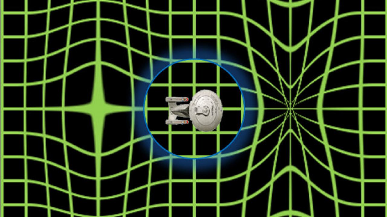
Figure 17: Alcubierre warp drive 'warping space'

Transformations of this kind can either be done on the object in question, in this case a spacecraft, or on the coordinate system surrounding them - in this case spacetime. And these transformations are logically considered equivalent. However, notice that in the case of the Mexican Hat diagram, no such transformational algorithm has been applied. Instead the shape simply falls out of the XNOR and XOR data, with the XNOR axis privileged in the y-axis and the inclusion XNOR variable (-1). This means that, according to the Dimensional Gate Operator hypothesis, this is truly the momentum-state information of our particle. This is what the wave function of our photon looks like when it is travelling at light speed. This is a remarkable confirmation, in my opinion of the concepts set out early on in this paper.

If indeed this is an accurate depiction of the momentum-state of the particle, then there are numerous conclusions that we can draw from it. First, we noticed the similarity between this graph and the Alcubierre warp drive. This drive is said to function on negative matter, or exotic matter. Some researchers have postulated that Dark Energy and Dark Matter may be a kind of negative matter that is driving the expansion of the Universe. If this is correct, then it would appear that the arithmetic of the Dark Matter Universe is XNOR. When we add a positive number to a positive in XOR we get a positive. But doing the same thing in XNOR gives you something negative. This in itself is a good description for negative matter and since the momentum-state of the particle appears to be represented in XNOR, it would appear that all matter has a dark matter component to it.

This could potentially gives us a way to test dark matter theory.

Next, we examined the notion of negative energy distorting spacetime and how this is equivalent to distorting the metric coordinate system. Notice how there is no distortion of the metric in the ‘Flattened Mexican Graph’. This means that what we are seeing here is more a kin to a traditional Doppler Effect. We can apply the same perspective to our more complex wave function of the photon.

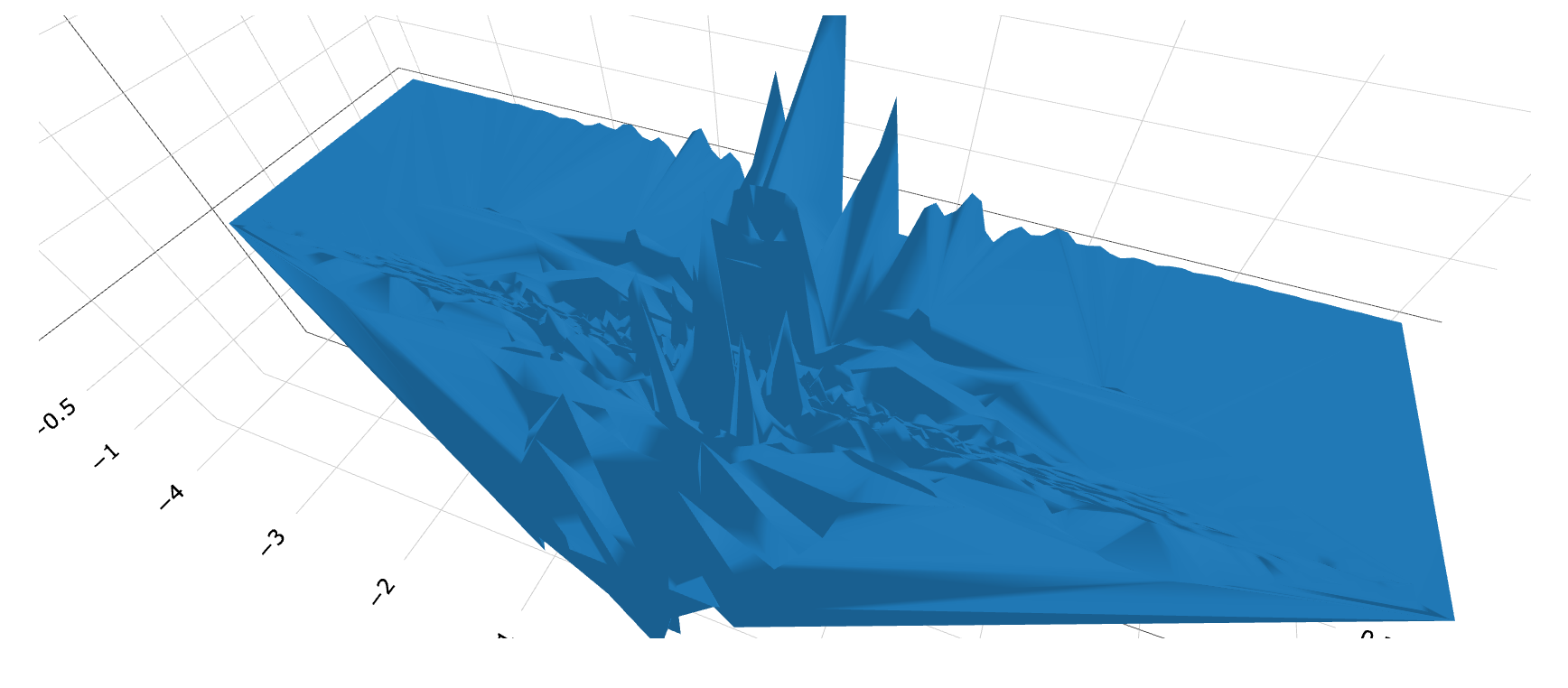
Figure 18: Photon moving and exhibiting Doppler Shift

The image above shows us a slice of what photon looks like in 4-D XNOR space. It has a pressure front and a wake. The fact that this can be derived without recourse to relativistic motion, suggests that it is entirely non-relativistic in character.

Conclusion

It would appear that using the XNOR logic gates in place of imaginary numbers we can reproduce some of the results we see from experimentation. So there is a relationship between the mathematics of XNOR space and particle physics. I think the method provides good insight into these quantum systems.