Dimensional Gate Quaternion Multiplication, Quarks & Polyhedra

Christopher C. O’Neill

chris.ozneill@gmail.com

10 December 2020

Abstract

Using Quaternion Multiplication, and the methods of Dimensional Gate Operators, we can construct various polytopes, including; rhombic dodecahedra, rhombicuboctahedra, cubes and their various polyhedral composites. The relevance of this method to Quantum Mechanics is further explored and discussed.

Keywords

Quantum Physics, Mathematics, QCD, Quantum Chromo Dynamics,  Quaternions, Quarks, Gluons, polyhedra, hyper-dimensional, 4D.

Introduction

The Universe is founded on mathematical principles. But what kind of mathematics? Is it algebraic? Or something else? Anyone with even a cursory familiarity with algebra knows that much of its application is in the area of determining the values of unknown constants and variables. This is incredibly useful from a human perspective, as it offers us a means to ascertain, what was previously unknown. But does the Universe operate like this?

Probably not.

The Universe already ‘knows’ the values of all the variables, it doesn’t need to find them out. That doesn’t mean that these constants and variables are not handled in the manner which mathematics dictates they are. In fact, it is hard to see how it could be any other way. An important indication that this is the case are the repeated relationships between various mathematical principles and the results of experiment.

But the previous point still holds true. Just because we can’t determine the value of the square root -1, doesn’t mean that the Universe doesn’t implicitly know that value. Just because we don’t know the order in which two quaternions were multiplied to arrive at a particular value, doesn’t mean that the Universe is not aware of it. In fact, if quaternions are a feature of the Universe — and a large amount of research into Quantum Physics would suggest that they are — then the Universe is constantly availing of this 4-dimensional space and has a complete record of all operations in said space.

Not so for us humans. In order to deal with the confounding nature of imaginary and complex numbers, we are forced to use algebraic placeholders like ‘i’. As we increase the dimensions, so the number of our placeholders increase, to include; j, k, and e_n. In order to get a handle on these unknown variables and their lack of order and commutativity, we need to translate them into Norm Division Algebras. But the number of these algebras increases with each step. There are Exceptional Lie Algebras and Clifford Algebras, Exceptional Jordan Algebras, not to mention the endless relationships between these and rotation matrices like O(n), SO(n), U, SU2, SU3, 5 and so on.

All of a sudden, it appears that our tools for understanding the Universe are becoming more of a hindrance than a help. Perhaps, we should consider that while Norm Division Algebras are crucial for how humans understand and do mathematics, they might not be crucial to the Universe, which already knows all of the aspects of itself that we wish to learn.

In ‘Reimagining Complex Numbers’, I showed how there exists another equally valid way to do arithmetic that allows for √-1 to be a real numbered value, without the need for arbitrary square operations. I also showed how it is possible to describe what is going on in the Complex Plane without the need for algebraic placeholders like the letter ‘i’, and which has no reality in the physical world.

To clarify, I am not suggesting that Complex Numbers and other higher-dimensional algebras like the Quaternions and Octonions should be abandoned. On the contrary, complex numbers are absolutely invaluable in many areas of mathematics, physics, chemistry, and engineering and their mystery and usefulness will never be diminished. Furthermore, I think it is best to avail of all the tools in our mathematical toolbox.

Therefore, I have decided to apply the rules of Dimensional Gate Operators to the Quaternions to see what will emerge. This method should allow us to use the Quaternions directly, without the need for complex, esoteric and laborious mappings to one of a growing number of exceptional algebras and the results could lead to a much broader area of research  and applications in the area of Quantum Physics.

Quaternions to the Present Day

Quaternions were invented by Irish Mathematician William Rowan Hamilton in the 1840s. Hamilton spent a great deal of energy promoting his new mathematics, by getting it recognised in journals and even going as far as to set up his own school of mathematics, where the principles of Quaternions were taught. But despite his best efforts, the method did not catch on. Simply put, no-one knew what to do with these strange 4-dimensional numbers. They couldn’t be easily multiplied or divided and so they remained fallow, lying in the dusty toolbox of forgotten mathematics.

Then, around a hundred years later, a very interesting thing happened. The Theory of General Relativity emerged and announced that the material of the Universe was a stretchy 4-dimensional spacetime fabric. Now, there was suddenly a need for a 4-dimensional algebra to describe this new space time. And out of the shadows, stepped the Quaternions…

Since, then the Quaternions have been used in many applications to do with General Relativity and Quantum Mechanics. But is perhaps in the latter that they have achieved the most success. The importance of vectors, eigenvectors and eigenvalues in late 19th Century mathematics made certain that the Quaternions could be used as a kind of four-dimensional vector.

Vector Quaternions

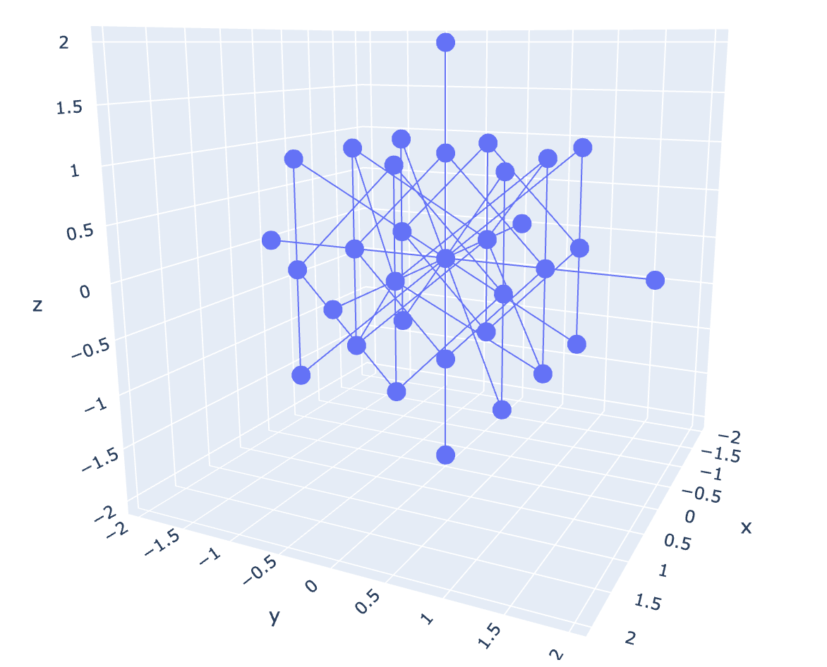
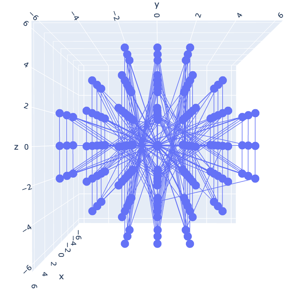
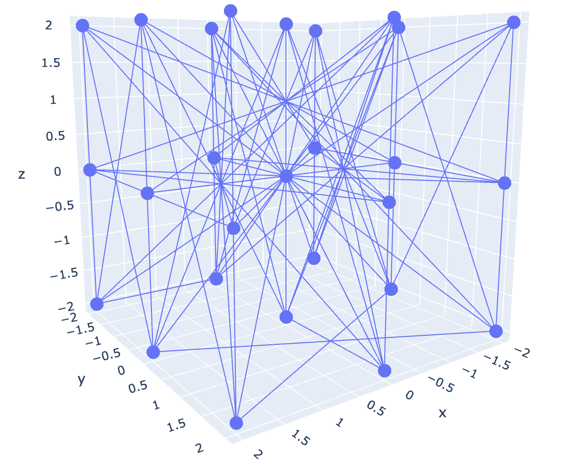
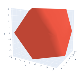
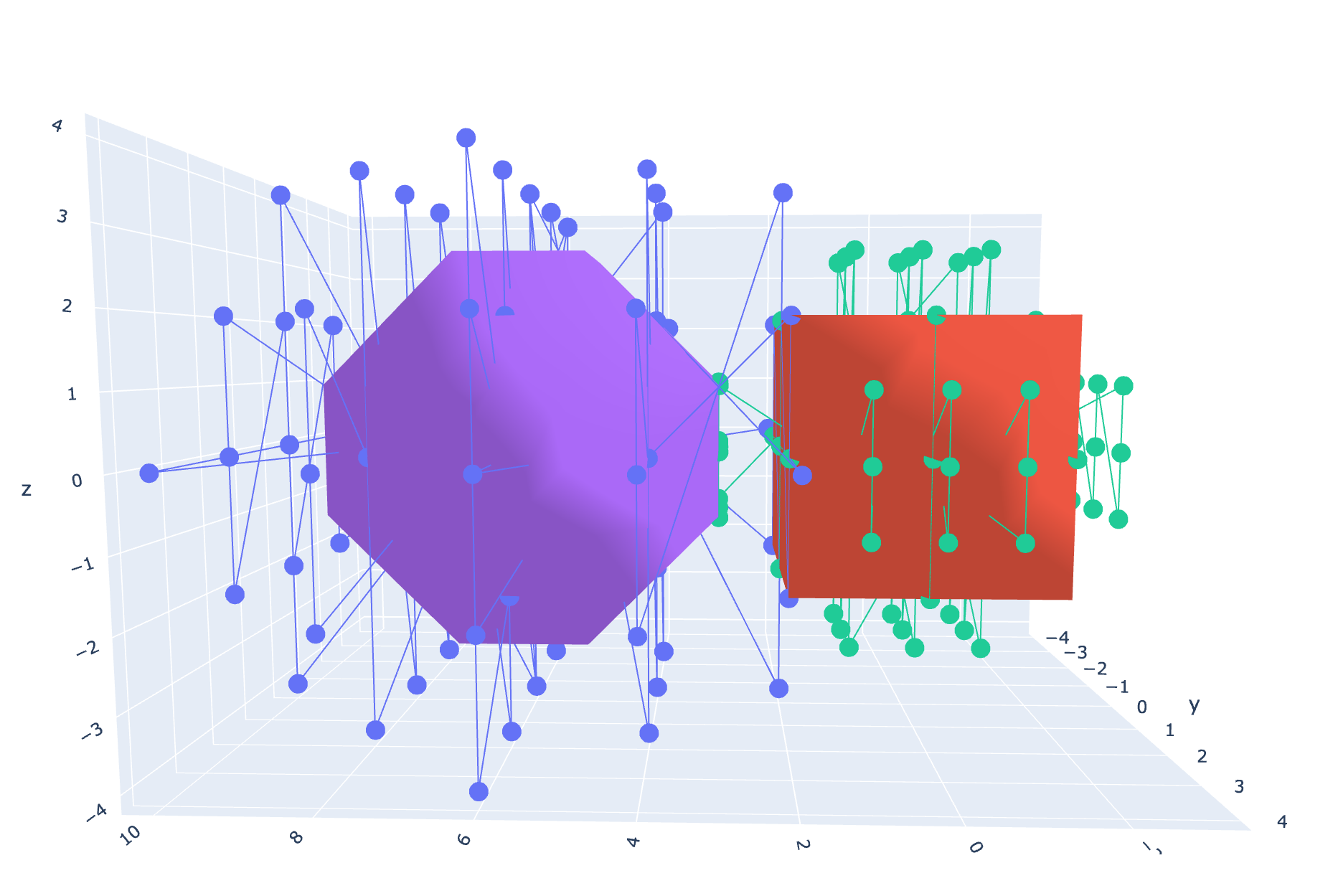
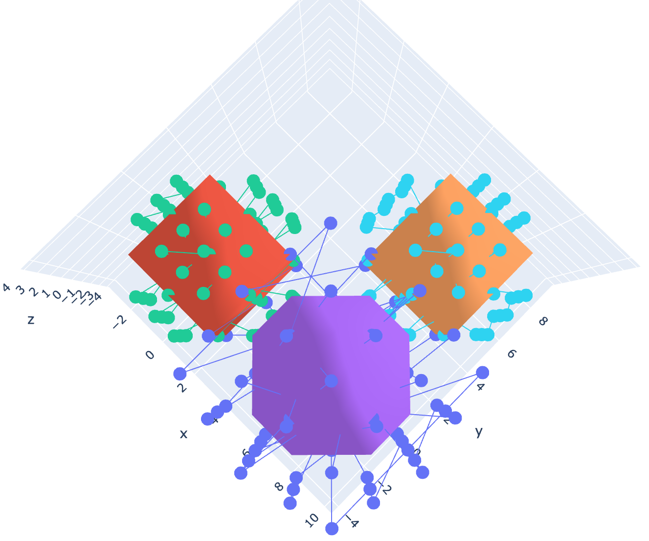
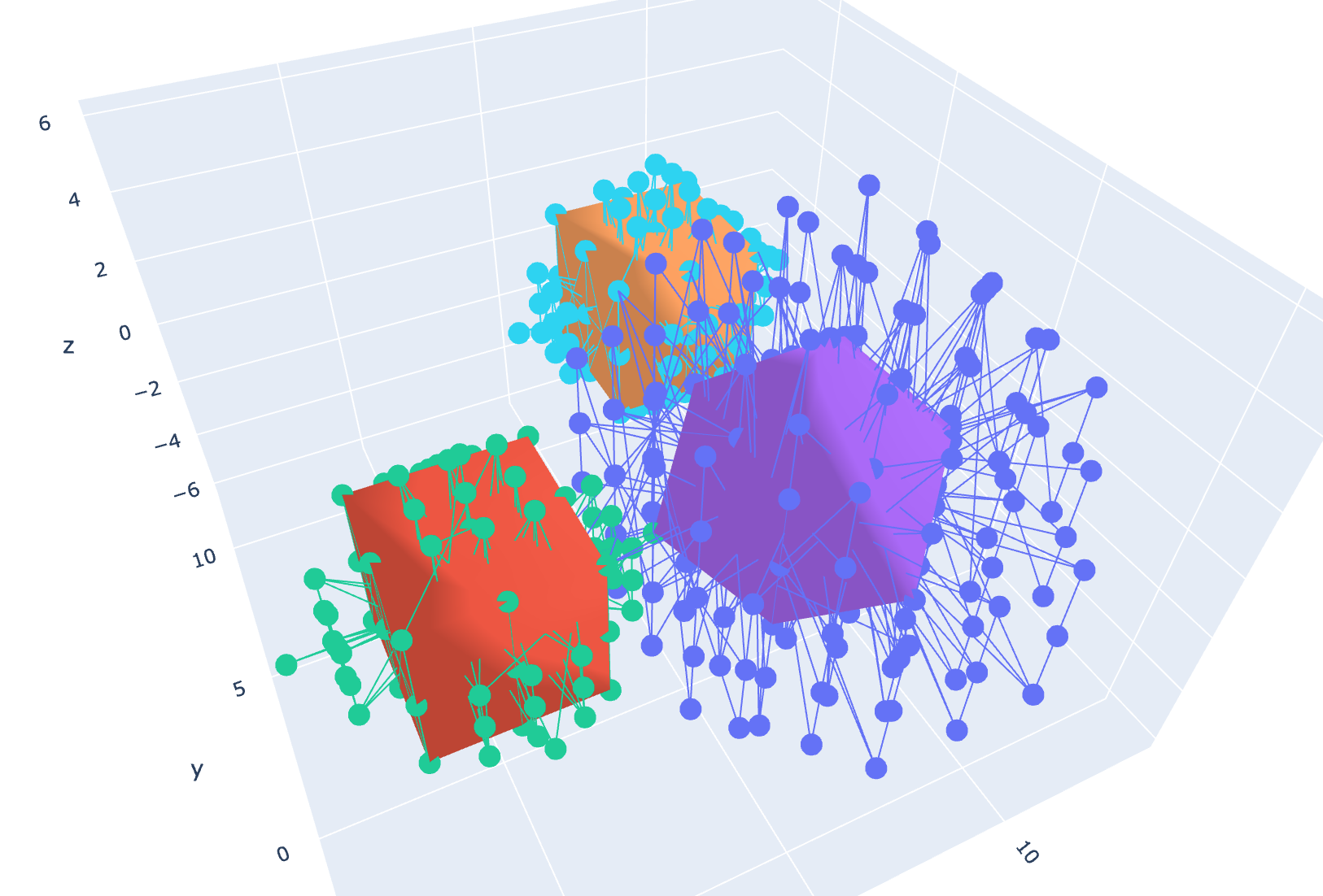
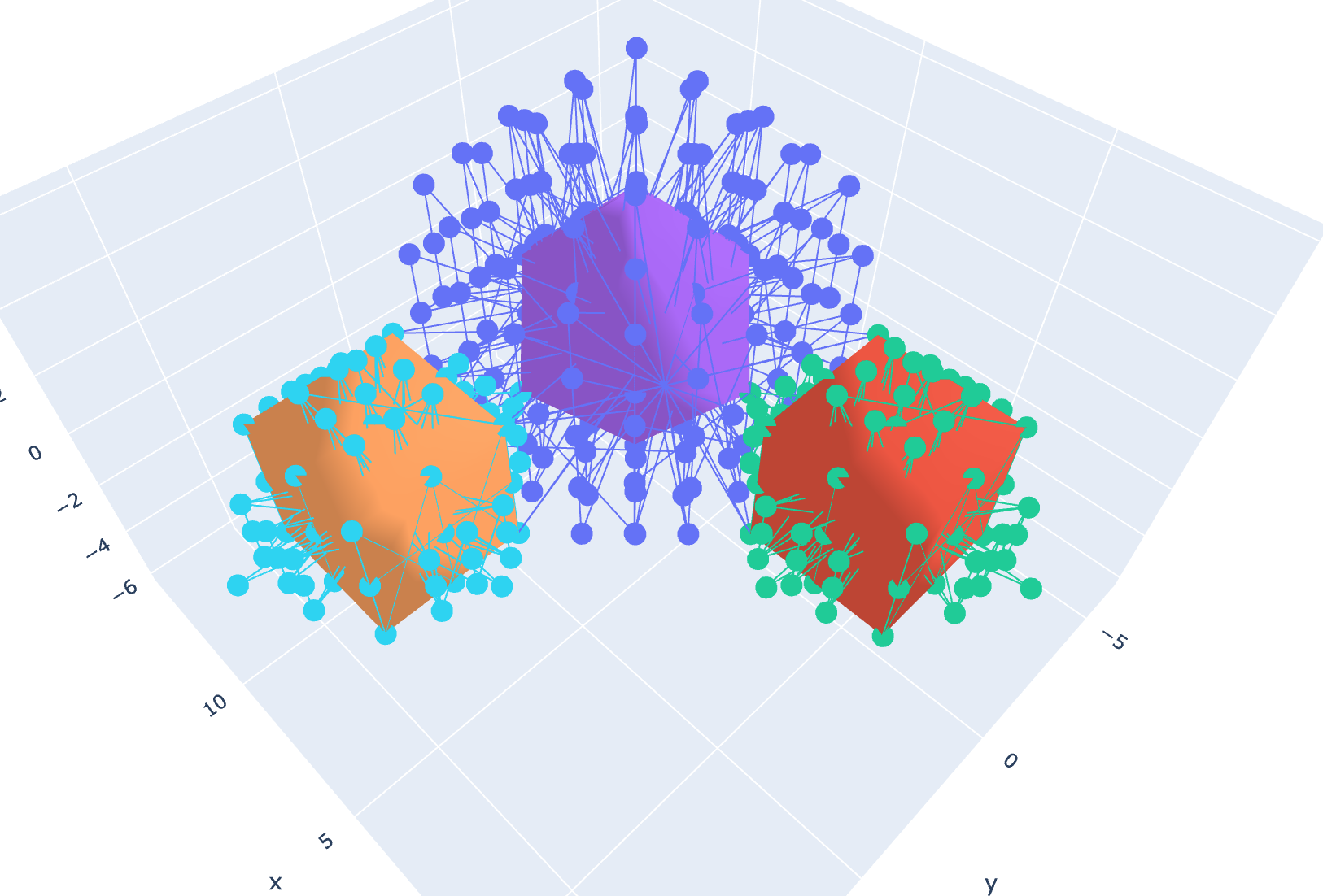
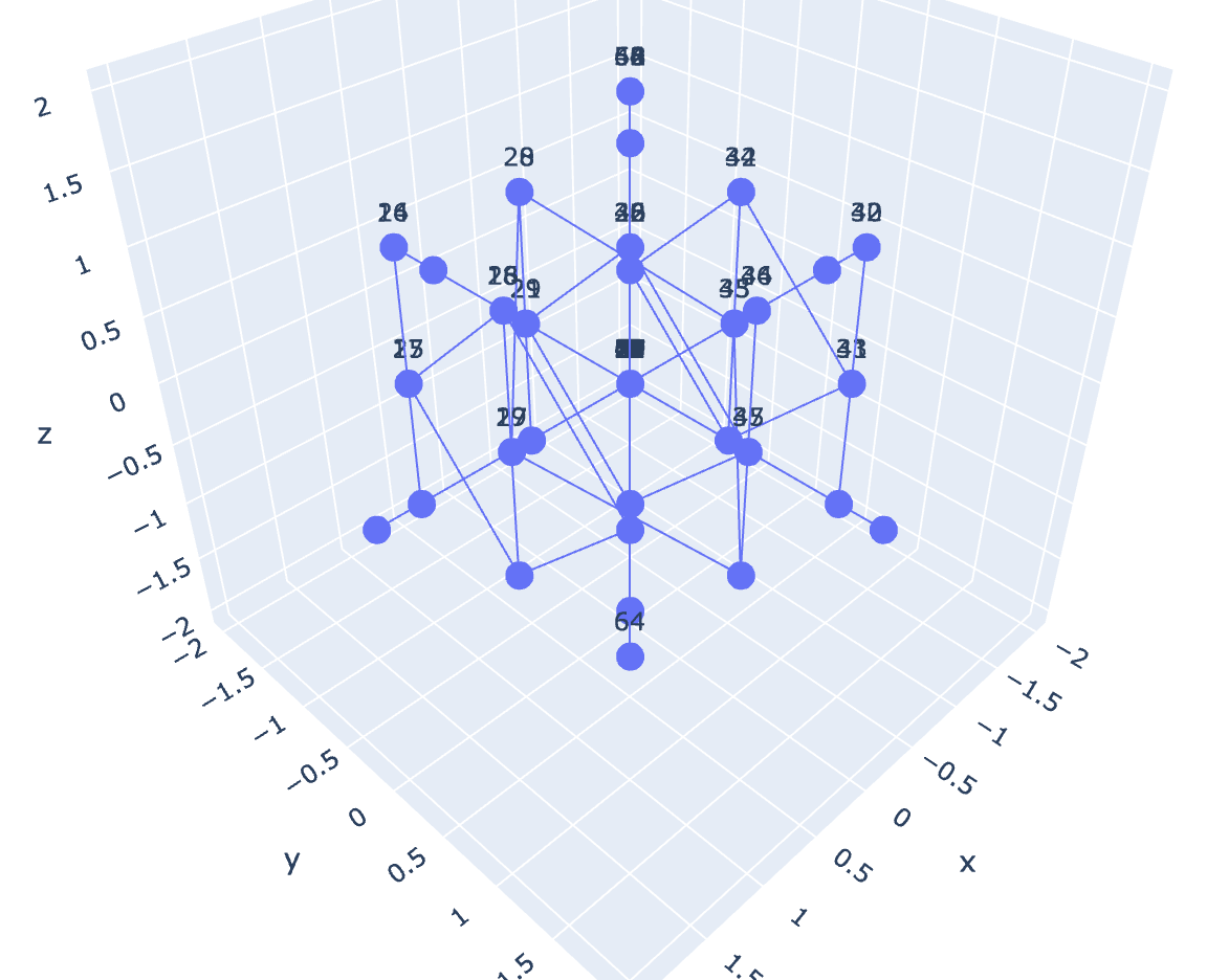
If we define a set of quaternions v(a, b, c, d) and multiply them by a second set of quaternions v(e, f, g, h) over a range of real numbers, we can produce a total of 8!/3!(8!-3!) = 56 unique perspectives on this four-dimensional object. Most of these perspectives are of interest to no-one. For instance, if we were to simply plot the vectors b, c, and d, we would only fill the space with numbers in a uniform and uninteresting way. But, if we just focus on graphing f, g, h, something very interesting happens:

Fig 1. DGO Quaternion multiplication over the range(-2, 2).

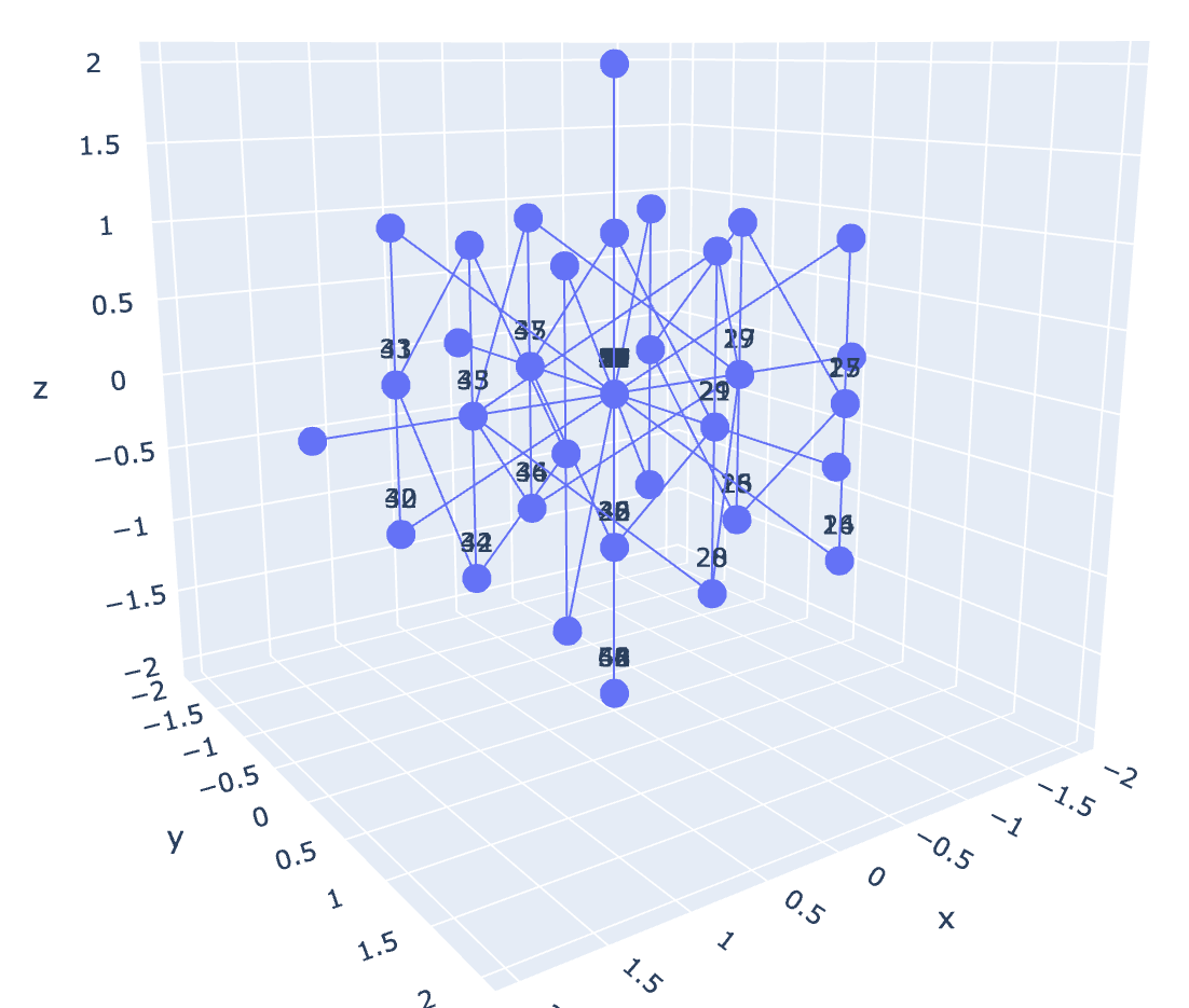
We get a discrete form…

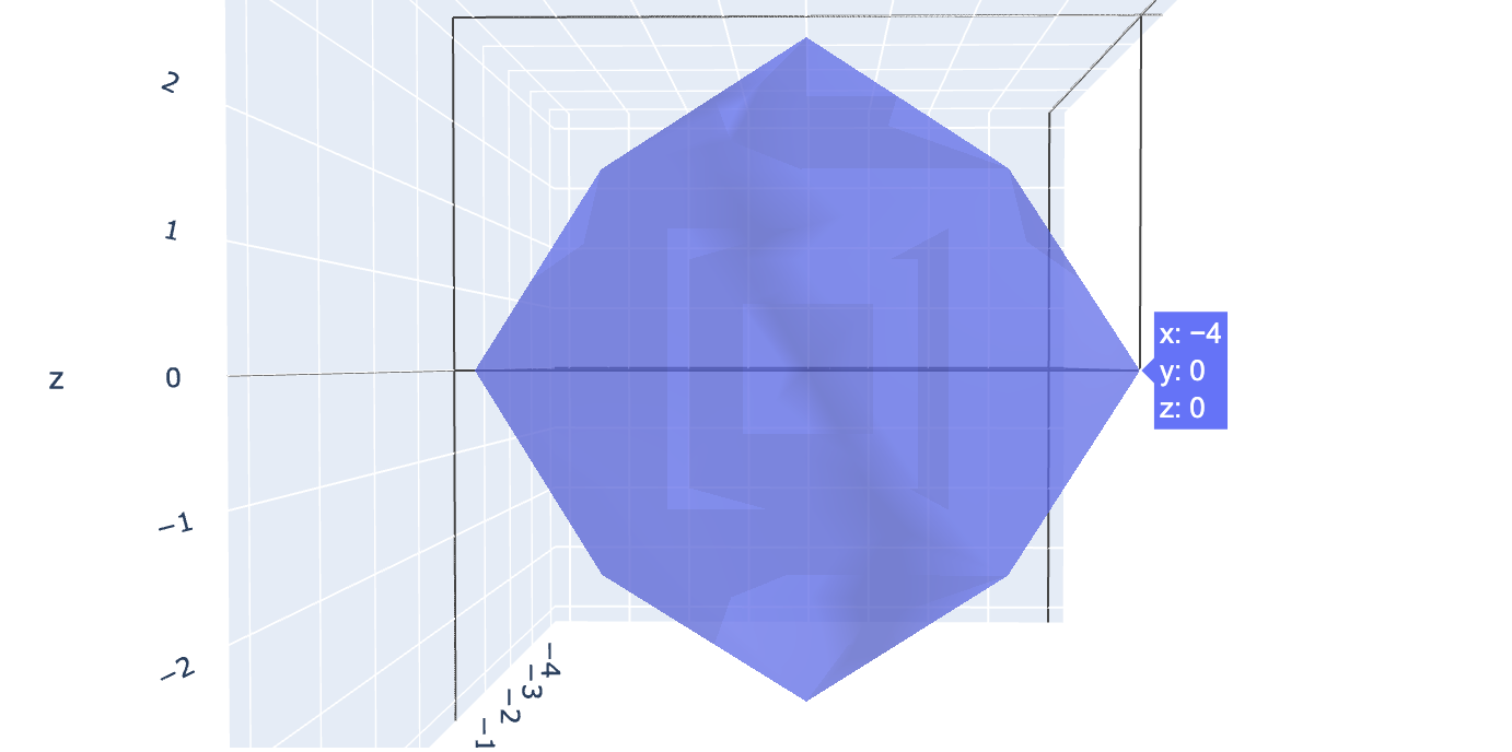
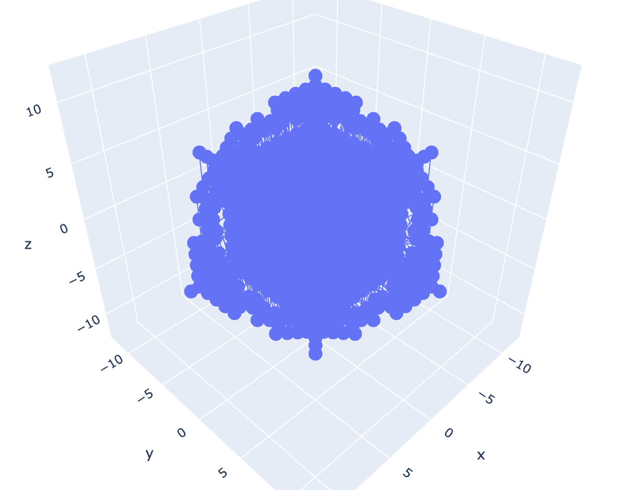
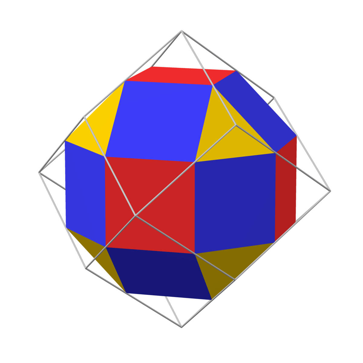
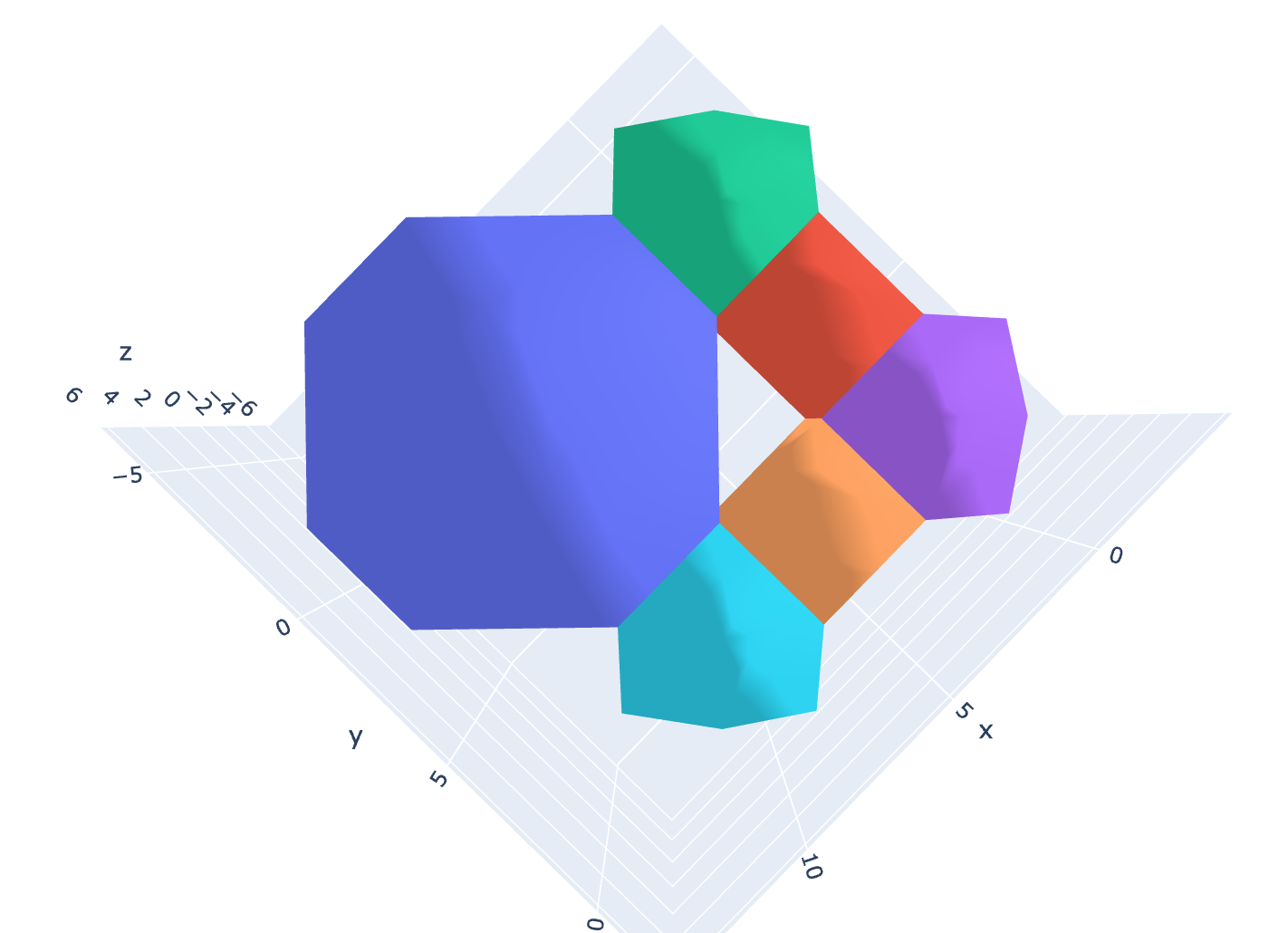
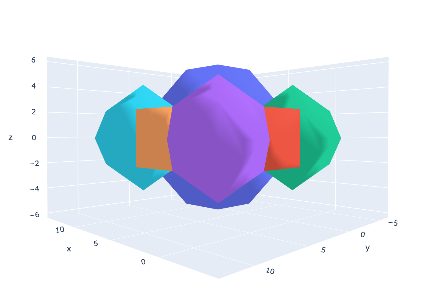
Fig 2. Alphahull = 0 of Fig 1 reveals a rhombic dodecahedron.

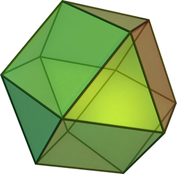
And not just any form, by applying alphahull=0, we can see (at least partially) that this is a rhombic dodecahedron (or rather a 4-dimensional rhombic-dodecahedron). The rhombic dodecahedron is the eighth Catalan Solid. It has 12 faces, 24 edges and 14 vertices. Koch and Koch have also derived Catalan solids from Coxeter 3d root systems using Quaternions. But I wonder if this is really a surprise, seeing as how the maps for these solids are implicit in the root systems.[1] Simply by multiplying two quaternion vectors together over a range of values and graphing their results, we can construct a Catalan Solid, without any need for Coxeter symmetries. This requires no extra math other than the quaternions themselves. It simply drops right out of the computation.

This implies that the eight-fold symmetries of the Catalan solids are somehow implicit in the mathematics of the Quaternions. If that’s the case, then perhaps the raw Quaternions aren’t as disordered as they appear to be.

Fig 3: The ordinary XOR Quaternion matrix (left) and the XNOR Quaternion matrix (right)

Anti-Quaternions

We have seen what Quaternions are capable of doing on their own. Now, let us consider what happens when we apply the logic of DGO. First, we define our expression. I’m using ‘•’ as the matrix multiplication operator:

(a1+ bi + cj + dk)•(e1 + fi + gj + hk)

Using the XNOR table in Fig 3, we get:

-ae - af(i) - ag(j) - ah(k)

-be(i) + bf - bg(k) + bh(j)

-ce(j) + cf(k) + cg - ch(i)

-de(k) -df(j) + dg(i) + dh

These are the Anti-Quaternions.

Notice how their matrix for is identical to the form in the !∆ table in Fig 3. This is a very useful bit of information and a handy shortcut for Quaternion matrix multiplication, of this type.

Summing these and graphing the Anti-quaternion four vector over a range of (-1, 1) gives us a scatter plot with 33 data points (see Fig. 4). You might be tempted to try and fit the 32 known subatomic particles into this framework and call it a day, as I was tempted to do. But, the truth is that this figure has far more than 33 data points. All in all, it has 256 overlapping points. This works out as 7.7575… values per unique data point, although it is clear that they are not evenly distributed.

256 or 8^3 is the result of the cubic multiplication that is going on here. A similar story occurs when we set the range to (-1, 2), which has 6561 (9^3). However, setting the range to (-2, 2) gives us 65536, which is 256^2 (See, Fig. 4). So, perhaps it is the squares and not the cubes which are important here. In this case it’s 16^2, 81^2 and 256^2, respectively. Once again, we see that the Anti-Quaternions traces the rudimentary form of the hyper-rhombic dodecahedron.

Fig 4. Anti-quaternion multiplication over the range(-1, 1) creates a rudimentary rhombic dodecahedron with 33 points and 256 data points.

The number 256 is interesting from the point of view of 4 binary bit multiplication. Considering that XNOR and XOR are two of these binary bits, this number is suggestive of some kind of binary informational code stored within the rhombic dodecahedron. A similar code has been posited for Quatum Computing in this paper [4].

Fig 5. Anti-quaternion multiplication over the range(-1, 2) once again reveals the Catalan Solid and has 6,651 data points.

My reason for displaying Fig. 5 is simply to give you an idea of how the Anti-Quaternion looks over a different range and because it reminds me of the Mandelbrot Fractal.

Fig. 6: Mandelbrot Set (Source: http://paulbourke.net/fractals/mandelbrot/)

As a matter of fact, the quaternions have been recruited to graph Mandelbrot Set and Julia Sets, to create the kind of geometry, which —as M.C. Esher would say — is both beautiful and disgusting, all at the same time.

The Next Phase

The next phase of the DGO is to add the XOR Anti-Quaternions to the XNOR Quaternions. Because these are two different systems, they must first be added in XOR and then in XNOR and finally summed together in XOR. In the case of Anti-Quaternions, the values i, j, k, which represent the √-1 become 1. And the complimentary values of the ordinary Quaternions become -1. When these two systems are summed together, we get the following two matrices:

Fig. 7: The different sums of the Quaternions (LEFT) and the Anti-Quaternions (RIGHT)

When the two resultant matrices are summed together we simply get our original Quaternion matrix multiplied by 2, which will obviously graph as another, bigger rhombic dodecahedron. But, before we do that we can go ahead and graph the quaternions on the left (in Fig 7):

Fig. 8: +∆ sums of the Quaternions and the Anti-Quaternions over the range(-1, 2).

And the Quaternions on the right produce the following graph:

Fig. 9: +!∆ sums of the Quaternions and the Anti-Quaternions over the range(-1, 2).

The alphahull of the graph in Fig. 8 produces a rhombicuboctahedron, whereas the alphahull=0 for Fig. 9 produces a cube. The rhombicubotahedron is the 10th Archimedean Solid, whereas the humble cube is the second Platonic Solid. At this point, whether we plus or minus these two solids from one another it will make no difference. They will both be a rhombic dodecahedron. It is interesting to note however that the 10th Archimedean Solid minus the 2nd Platonic Solid equals the 8th Catalan Solid; 10 - 2 = 8. It would be interesting to see if this pattern can be recreated with other solids of their kind in Quaternion space, although I suspect that this is the sweet spot as far as Solid (or Polyhedral) Arithmetic goes.

It may also be worth noting, for now, that the Rhombicuboctahedron embeds inside the rhombic dodecahedron. This allows us to add polyhedra in different ways to create new composite polyhedra.

Fig. 10: Rhombicuboctahedron embedded in rhombic dodecahedron (Source: https://commons.wikimedia.org/wiki/File:Rhombicuboctahedron_in_rhombic_dodecahedron.png)

Since we have already determined that polyhedra are the natural shape of the Quaternions and the Anti-Quaternions, what can we say about these shapes and their applications? The obvious place to start is in the zoo of quantum particles. Is it possible that the simple multiplication of DGO Quaternions results in the creation of subatomic particles?

And if so, which ones?

Particle Soup

Initially, I was tempted to class the rhombic dodecahedron as a quark and the cube and the rhombicuboctahedron as gluons. But, after further research, I have decided to switch these around. The reason for doing so is 2-fold. The first consideration was based on the (rest) masses of the gluons and the u and the d quarks. The d quark has a mass of 4.7 MeV/c², where as the u quark is only 2.2 MeV/c². The mass of the gluon is unknown to any degree of certainty. To quote Wikipedia, it is “less than a few MeV”, so we’ll say that it lies somewhere between 2.2 and 4.7.

The number of unique points in the Rhombic-dodecahedrons (seen in Fig. 4) is 13. The cube based of this has 9 and the Rhombicuboctahedron (RCO) has 37 unique points. Their total number of points is 33, 27, and 106 respectively. Notice that the RCO is much larger than the others. It is in fact twice as large. As a consequence it can’t be graphed over the usual range of (-1, 1), it needs extra room. If we were to liken the number of points to the mass of the object, then it is clear that the cube is the lightest, the rhombic dodecahedron is heavier, and the RCO is the heaviest.

Assigning each of these polyhedra a particle based on their sizes then becomes trivial. The rhombic dodecahedron is the gluon, the cube is the up quark and the RCO is the down quark.

Fig 11: The Octonions in their traditional algebraic form.

The second reason stems from the structure of the Quaternions themselves. Hamilton’s complex domains can only be constructed in powers of 2, so; 2^2, 2^3, 2^4 and so on. This is a consequence of the underlying algebra. There is a gap between the Quaternions and the domain of the Octonions and an even larger gap, between the Octonions and the 16-dimensional Sedenions.

But, it is clear that we can have 5 quaternionic vectors, if we simply take 5 octonions at a time. There is no reason why we can’t do that, according to DGO, since we have long since dispensed with the algebraic values i, j, and k, in favour of 1 or -1. Graphing the Hamilton Product of two 5D Quaternions (Pentonions), over the range (-4, 4) produces an RCO, with 59049 data points.

Fig 12: An example of a real number valued Pentonionic matrix.

This is rather a large beast. My computer refused to calculate the 6-dimensional version of the quaternions — it was simply too much work. But I was able to get enough information out of it to conclude that the 6D Quaternions (or Hexonians) produce a rhombidodecahedron again. Based on this pattern, it would appear that the RCO is related to odd numbered values and the rhombic dodecahedron to even ones.

While I can’t calculate further than that, at the moment, we can continue the same process in reverse. Removing one degree of freedom from the Quaternions, gives us the Trionions, which once again produces an RCO, when graphed. Dropping down to just two degrees of freedom (Dionions) gives us the geometry of rhombic dodecahedron again, so at this point, I’m confident the pattern is confirmed.

Where have we seen this pattern before?

That’s right, in both the section entitled Anti-Quaternions and in the Next Phase where successive ∆ and !∆ quaternions were added together. This gives us an entirely new way of generating new generations of spin-1/2 particles. Which of the methods yield better results, as it pertains to the masses of these particles, is still a matter of study. But preliminary results show that Pentonion RCO has 59049 data points, while its Quaternion counterpart summation of the XNOR and XOR quaternions only has 6561. This is a 9-fold difference.

Dionion and Trionions

Since dionions are only two-dimensional they produce some strange behaviours when graphed. But, since the probabilities of the spin states of particles are calculated using two-dimensional Pauli Matrices, they can hardly be overlooked.

Fig 12: An example of a real number valued Trionion matrix.

For instance, altering the perspective of the Dionion multiplication, which is easy to do, gives us a wave function with some interesting characteristics. It should be noted that this is simply the top level of the wave function, it is many layers deep.

Fig 14: Dionion wave function. Possibly related to gluon field.

If our assumptions about rhombidodecahedron being the shape of the gluonic field are correct, then the images in Fig. 14 and 15 may represent something of the character of the wave function.

Fig 15: Dionion wave function 2.

But, I don’t want to play around with two-dimensions currently. I want to explore the rhombic dodecahedron and RCO in higher dimensions. To keep things simply, and reduce processing time, we’ll just stick to the Trionions, or just 3 dimensions, for now.

You might be forgiven for thinking that the sum of the ∆ and !∆  RCO equal a cube and a rhombic dodecahedron, as I did. If you did, you were half right. This time the XNORed value is the cube and the XORed value equates to cuboctahedron, which is the dual of the rhombicuboctahedron.

Fig 16: Cuboctahedron

Now, our gluons are rhombicuboctahedral, our u quark is still cube-shaped and our d quark is a cuboctahedron. To create a pion (π) — plus or a minus, it doesn’t matter — we simply need to bring the u and d quarks together with a gluonic field. This results in Fig. 17.

Pions are highly unstable, but it is hard to see from this graph precisely what makes them unstable. Perhaps by graphing a proton, we might get a better understanding. In Fig. 18, we see two u quarks and a d quark together with their gluonic fields. There is nothing that I can see that would be more ‘structurally sound’ in this model. But perhaps going back and graphing it in the 4-dimensional Quaternions would give us a better indication.

Fig 17: Two trionion fermions coming together to form a boson.

In these examples, I’ve switched between Mesh and Scatter graphs, to allow you to see how the polyhedra connect. 

Fig 18: Trionion proton formed from 2u and 1d.

Using this method, it is not difficult to see how neutrons and other nuclei like pentaquarks could be constructed. But in order to do that we have to have a solid basis for constructing anti-quarks and the various colour charges. Note that in Fig. 18 the red and blue gluonic fields don’t connect. This is a because I have represented the quark and gluon fields as overlapping.   In reality, they should most likely not be. They should alternate; quark, gluon, quark, gluon etc. forming a ring.

For the sake of completeness and accuracy, I have decided to model the Quaternion version of a proton (Fig 19 and 20). This shows the gluons as hyper-rhombic dodecahedrons, the u and d quarks as cubes and RCOs, respectively. I’ve also included the alternative or ‘ring’ version of the proton (Fig. 21 and 22). [5]

Fig 19: Quaternion Proton formed from 2u and 1d.

Fig 20: Same as above, but from a different angle.

If the thought of quantum fields existing as perfect cubes in space has you scratching your head, then you’ll definitely enjoy Baez’s excellent blog post on quantum fields (in this case atomic orbitals) being expressed as Platonic Solids. [5]

Fig 21: Alternating quark gluon quaternion model.

Fig 22: Different angle of above

Standard Quarks

There are three generations of quarks and anti-quarks, making a total of 12 quarks. There are six colour charges, 3 of which are anti-charges. So, this makes 36 different types of quark. The colour charges red, blue and green are equivalent to spatial rotations (like; x, y, z). If we imagine that our Quaternion Up quark is ‘red’, then all we have to do to change its colour is to rotate it 90 degrees. All we have to do to convert a quaternion quark into a quaternion anti-quark is to multiply the matrix by -1. Summing this result with itself will result in a matrix of all zeros (total annihilation). But rotating any of these anti-matrices will produce a different matrix, which won’t annihilate and so that allows us to build mesons out of quark and anti-quarks, of different colours and flavours.

But hang on a minute… If the quark is a cube and which is symmetric under rotations of 90 degrees, then how are we to know that it is rotated? The answer to this comes from the underlying structure of the quarks.

Fig. 23: Up Quark, here represented for demonstration purposes as a rhombic dodecahedron.

In this example, the u quark begins construction in the positive upper half of the coordinate plane, before extending to the negative upper half. Whereas, the down quark, is the mirror image reflection of this (Fig. 23 & 24). The anti-red, anti-green and anti-blue colour charges result from similar rotations of antiparticles. Rotating an up quark along a certain axis has the ability to change a green to a red quark. Since gluons are primarily responsible for such colour changes, it is to be assumed that the rhombic dodecahedron (4D) or  the cuboctahedron (3D) plays a role in this rotation.

This is not too surprising, as we have already pointed out that the √2 and √3 are both aspects of the rhombic dodecahedron geometry. Less obvious is the fact that the G2 root system of SU(3) can be attributed both to gluon rotations and the 12 mid points of a cube or the vertices of a cuboctahedron.[2]

Now that we have 15 of the elementary particles sketched out, we can complete the entire set of quarks in the Standard Model, by generating two more generations. But how do we go about doing that?

One possible answer lies in the construction of DGO arithmetic.

When we multiply two DGO systems together, like ∆ and !∆, we can then sum the results of both operations using XNOR and XOR. This gives us two new results, which are summed finally with XOR to give us our answer. This works very well, in most cases. But it is obvious that there is no need to stop there, as we could simply continue summing our two answers with XNOR and XOR indefinitely. When this is done, the two systems begin to increase exponentially and each successive generation can be likened to a new energy level taking the ordinary up and down quark to the strange and charm quarks and finally to the top and bottom quarks.

Fig. 24: Down Quark; again represented as a rhombic dodecahedron.

In this way, we satisfy a complete catalogue of quarks, as described by the Standard Model. But surprisingly, we are not done, as the situation gets a lot weirder. If we examine this table in Fig. 23, we see that the sum of a matter/anti-matter particle in ∆ causes complete annihilation, as expected;

Fig. 25: Quark-gluon table.

However, this is not true, when we sum in !∆.  Instead it is the summation of the ups and the downs that annihilate. This is weird and suggests an entire set of particle interactions that we know nothing about. Either that, or it is describing the interactions of negative matter and negative anti-matter, which means that both of these properties are somehow intrinsic to how matter is formed or constructed. From this perspective, an anti-matter and matter particle annihilating in this Universe would form a meson in the mirror Universe and vice versa, verse vica, visa verca (for all four dimensions you understand). This might explain why mesons are so unstable, they only exist for as long as it takes the particles to eradicate…

In both, Fig 23 and Fig. 24, I had to represent the quarks as rhombic dodecahedron, as the numbers were too difficult to see and therefore less apparent in the RCO model. As we know, it is the cube that represents the u quark and the RCO that represents the d quark. More accurately, the u quark is a hypercube (tesseract) and the RCO is a 4-dimensional polytope known as a known as a ‘Rhombicuboctahedral prism’ (See Fig. 26).

Fig 26: A Quaternion down quark represented by a Rhombicuboctahedral prism. Image source: (https://en.wikipedia.org/wiki/Rhombicuboctahedral_prism#/media/File:Rhombicuboctahedral_prism.png)[3]

There is more to say about the implications of 4D shapes like this one with respect to Quantum Chromodynamics i.e. gluon colour charges. But that is a whole other complex field of study and is therefore deserving of its own treatment in a separate paper. This will likely be my next paper (Keywords: Quaternions, gluons, Quantum Chromodynamics and QCD).

Conclusion

There is obviously much more ground to cover in this investigation into DGO Quaternions, Dionions, Trionions and all the other Polyonions. So far, we have been able to dispense with an algebraic approach to the Hamilton Product of the Quaternions and thereby free ourselves up for rigorous investigation into the kinds of polyhedra that they naturally produce. Thus, we have been able to create; cubes, cuboctahedra, rhombicuboctahedra, rhombic dodecahedra, with the potential for many more polyhedra to be found inside the domains of the Polyonions. We have been able to assign comfortably 36 subatomic particles to the DGO Quaternion method, including potentially all three generations of quarks, along with their colour charges and associated masses and spins.

Citations

[1] Catalan Solids Derived From 3D-Root Systems and Quaternions, Koch  & Koch, https://arxiv.org/pdf/0908.3272.pdf

[2] An Exceptionally Simple Theory of Everything, Garret Lisi, https://arxiv.org/pdf/0711.0770.pdf

[3] Image Credit: (Robert Webb's Stella software: http://www.software3d.com/Stella.php)

[4] The surface code on the rhombic dodecahedron, Andrew J. Landahl, https://arxiv.org/pdf/2010.06628.pdf

[5] https://johncarlosbaez.wordpress.com/2017/12/31/quantum-mechanics-and-the-dodecahedron/