Imaginary or Real?

Imaginary numbers are invaluable in many areas of mathematics, physics, and, in particular, quantum mechanics. They allow us to extend our understanding of the real numbers into the abstract realm of the Complex Plane. Complex numbers are in the form of (a + bi), where ‘a’ and ‘b’ are real numbers (like; 1,2,3..) and ‘i’ is the square root of -1. The Complex Plane can be further extended into the 4-dimensional realm of the Quaternions, Octonions and Sedenions etc.

However, with each successive extension of the Real numbers into these imaginary realms, some functionality is lost. The Real numbers are very good at describing and modelling the world. This is because they are ordered, commutative and associative. When we move up to the Complex Plane, the numbers are no longer ordered. This is because the √ -1  is not a known value. When we reach the Quaternions, we lose the property of commutation. The situation gets worse as we go to the Octonions where the property of associativity is lost. Now, a(b*c) no longer equals (a*b)c. This makes it incredibly difficult to do actual calculations in these mathematical realms. In the 16-dimensional world of the Sedenions non-trivial division by zero is allowed.

So, where does all of this difficulty and confusion stem from? Obviously, it stems from the root of all of these mathematical spaces, namely; √ -1 . So what is √ -1 ? If we find the answer to that, we should be able to resolve all of these problems and advance our knowledge of number systems and the Complex Plane.

Real or Imaginary?

When we learn about imaginary numbers at school, we are asked to solve √ -1 , and when we fail to do it, we are informed that there is no actual solution. This doesn’t sit well with most people and it didn’t sit well with me, the first time I heard it. I couldn’t bear the idea that mathematics was unable to solve something so basic and the fact that this uncertainty extends into the higher dimensional complex space, just makes the situation even more untenable. Something had to be done.

And, of course, it was. Mathematicians are a clever bunch. They were able to multiply the complex number (a + bi) by its conjugate (-a - bi) to obtain the absolute value of any number in the complex plane. This result is possible because squaring √ -1  gives you -1. As a result some order is restored to the Complex Plane and we can begin to understand, at least in part, something of their enigmatic majesty.

But is there another solution to this problem?

Quite possibly. At this level of maths, multiple solutions abound. We just have to make sure that our axioms and assumptions are correct to begin with. Let’s try and solve √ -1  =i together. If i² = -1, then i*i=-1. If we substitute +1 for i we get +1, so that can’t be right. If we use -1, we still get plus one. So that can’t be right either. In fact no matter what number we use, we will never get i²=-1. So what’s the solution?

The solution is to change how the operators work. What do I mean by operators in this context? In mathematical language operators are those like; {+, -, x, ÷}. When we multiply a positive number by a positive number, we get a positive real number. When we multiply a negative by a positive, we get a negative and when we multiply a negative by a negative, we get a positive number. It is the first and last rule that prevent us from solving √ -1 . So what do we do? We change the order of the operators and how they work.

There are many ways to do this. The current arrangement of our operators is isomorphic with the XOR logic rule set — also known as ‘exclusive or’.1 Our resulting rule set looks like this:

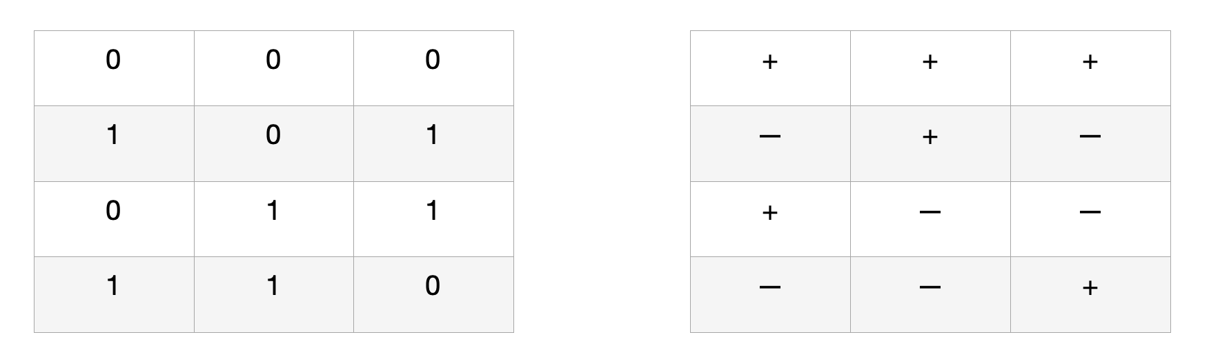
As you can see, the 0s and 1s of the XOR table exactly match the ‘+’ and ‘—’ of our operators. And this works equally well for the divisors. Why is our math based on the XOR system, you might ask? Why not on some other more familiar logic system, like OR, AND, NOR or NAND? It seems sort of arbitrary, doesn’t it?

While there are good logical reasons for why a minus multiplied by a minus equals a plus, it would appear that in the case of √ -1  the Complex Plane, this property no longer holds true.

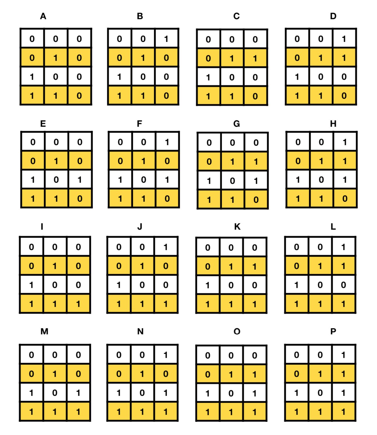
If we examine the logic chain for XOR, which is: 0110, we see that this is the binary number, which is itself equal to 6 (or 7 depending on how you count them). Since there are 16 variations on a four bit binary number, it is conceivable that we have 16 variations of our number bit operators and it is certain that our new set of operators are to be found there.

Notice how these 16-dimensions corresponds to the 16-dimensions of the Sedenion Numbers. But unlike, the n-dimensional division algebras of the imaginary numbers, these systems will be both well-behaved (ordered), commutative, and associative. Furthermore, they will permit extensions into odd and singly-even dimensions. In this sense, 5, 6 and even seven dimensional algebra will be possible in a manner that will be relatively simple and easy for anyone to understand. But before we do that we must choose our operator set.

So what is the best choice? Obviously one where positive square numbers and negative square numbers equal negative numbers. XNOR will easily achieve that. So, let’s set our Complex operators to XNOR, like so:

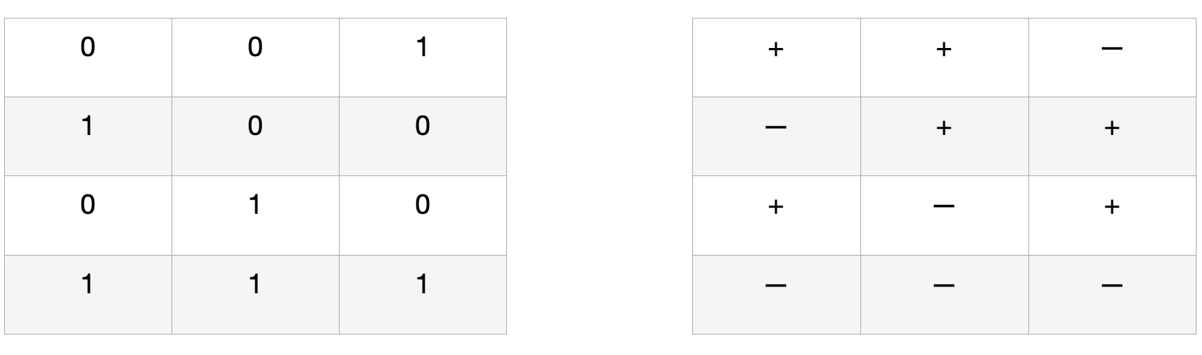
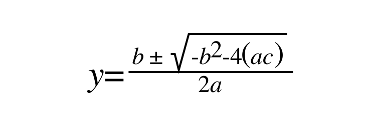
With this set of operators we can now easily prove √ -1  to be equal either to +1 or -1. Our next step is to privilege this result; meaning that from now on all of our mathematics will be done in the XNOR (!∆) operator set. When we do this, we inevitably find the somewhat perplexing value of √ 1 , which can’t be solved with our current operators. Our new XNOR equation for the quadratic formula looks like this:

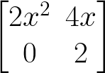
Using this to solve the equation 2x2 + 4x + 20 = 0, we get:

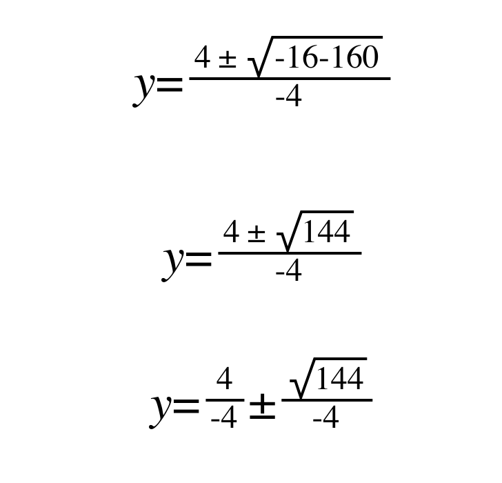
which is equal to 1-3i or 1+3i, where ‘i’ is the square root of 1. What’s the square root of 1 in XOR? Well, we already know this. It is ±1. Now, we have a complete and ordered set of operators for the complex plane and we can do algebra with it.

Suppose we want to plot: 2(3+i)(4+i). Under the original Complex Plane method this would lead to:

2(3+i)(4+i) = 22 + 14i

Under the Logic Gate Algebra, our original expression would be rendered in the form 2(!∆+3)(!∆+4); the terms are reversed, because we have privileged the use of !∆ (XNOR) over ∆ (XOR). The result of this is:

2(!∆+3)(!∆+4) = 22

This is much simpler and well ordered. But what is going on here?

When multiplying through the two different systems XNOR and XOR, we have to multiply the terms twice, once in each system. This generates two equal results of opposite signs, which then cancel each other out.

2(!∆+3)(!∆+4)

2(-1 + (4-4) + (3-3) + 12)

2(-1+12) = 22

This is equivalent to multiplying FL instead of the full mnemonic: FOIL, which stands for (First, Outer, Inner, Last). But we can’t expect this to work with larger expressions like (!∆ + 1),³ or (!∆ + 1)⁴ and so on. New rules must be developed for each. Alternatively, they can be placed into matrices where the values cancel out to zero and the remainders are summed to give the answer. If we were to simply graph 2(x+3)(x+4) on a normal Cartesian graph, we would get the familiar quadratic curve:

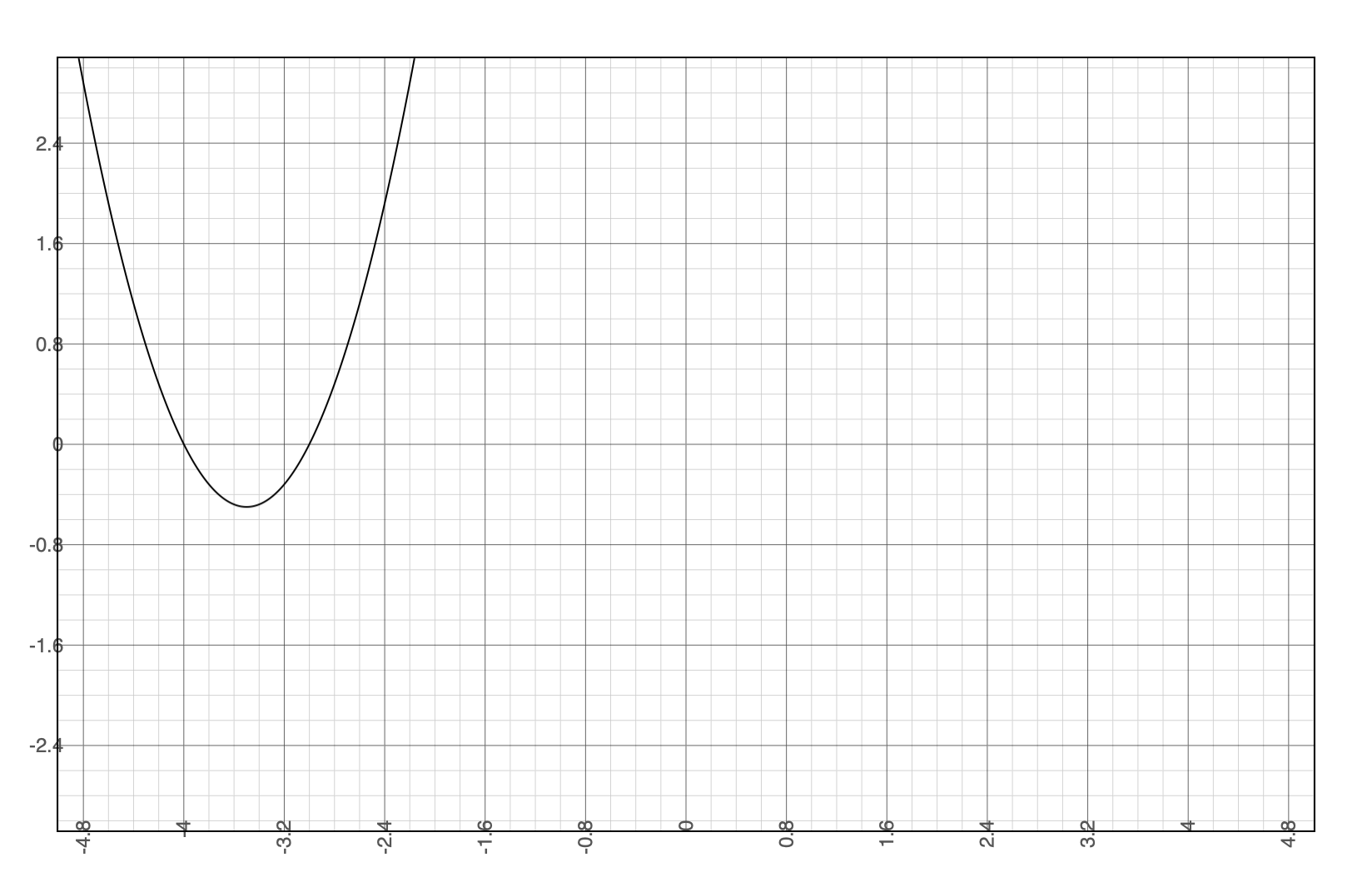
Figure 1: 2(x+3)(x+4) quadratic

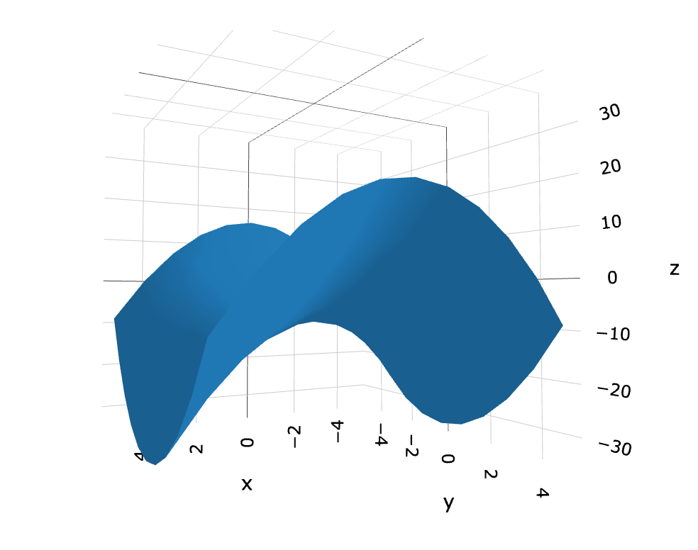
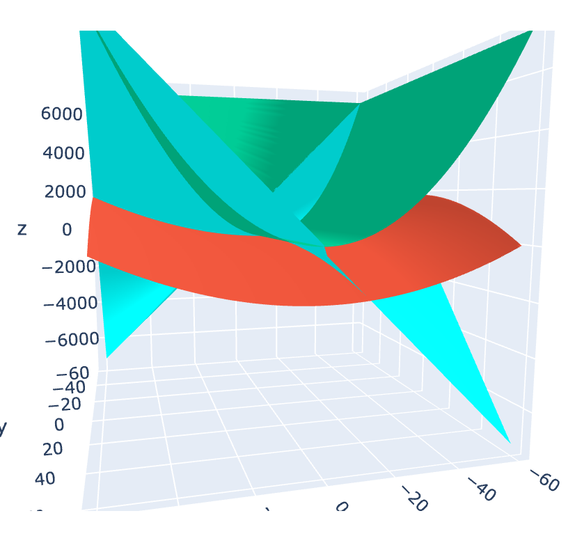
Plotting the same function in 3-d using a plotting program, gives this similar, but not so amazing result:

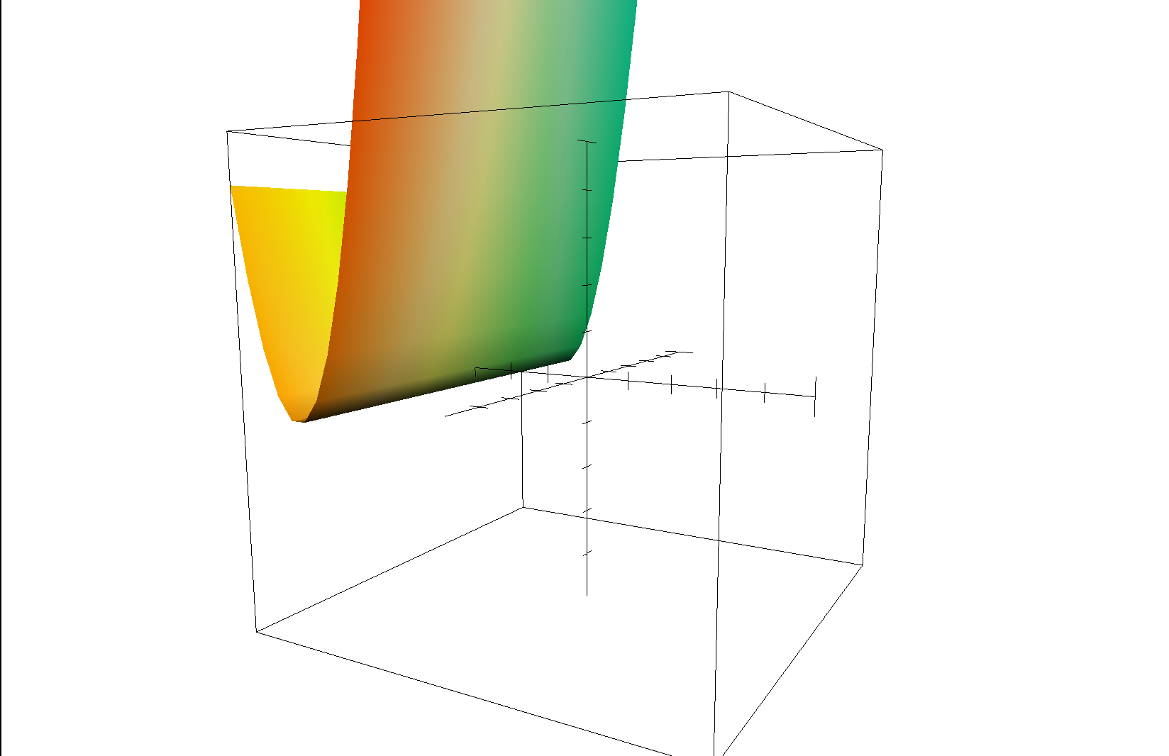
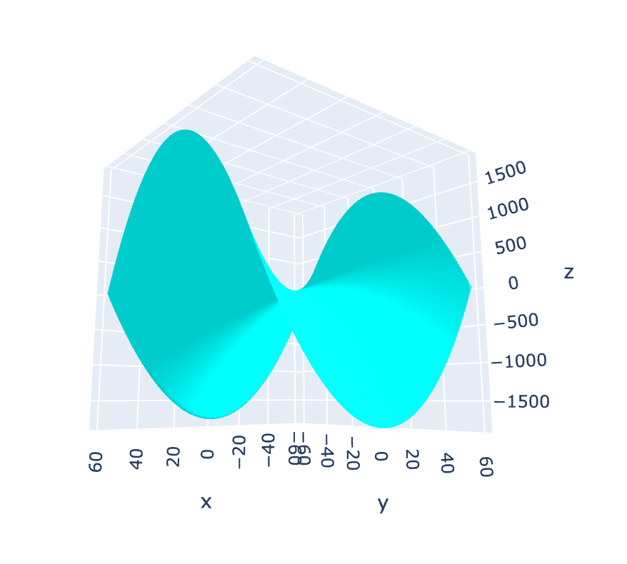
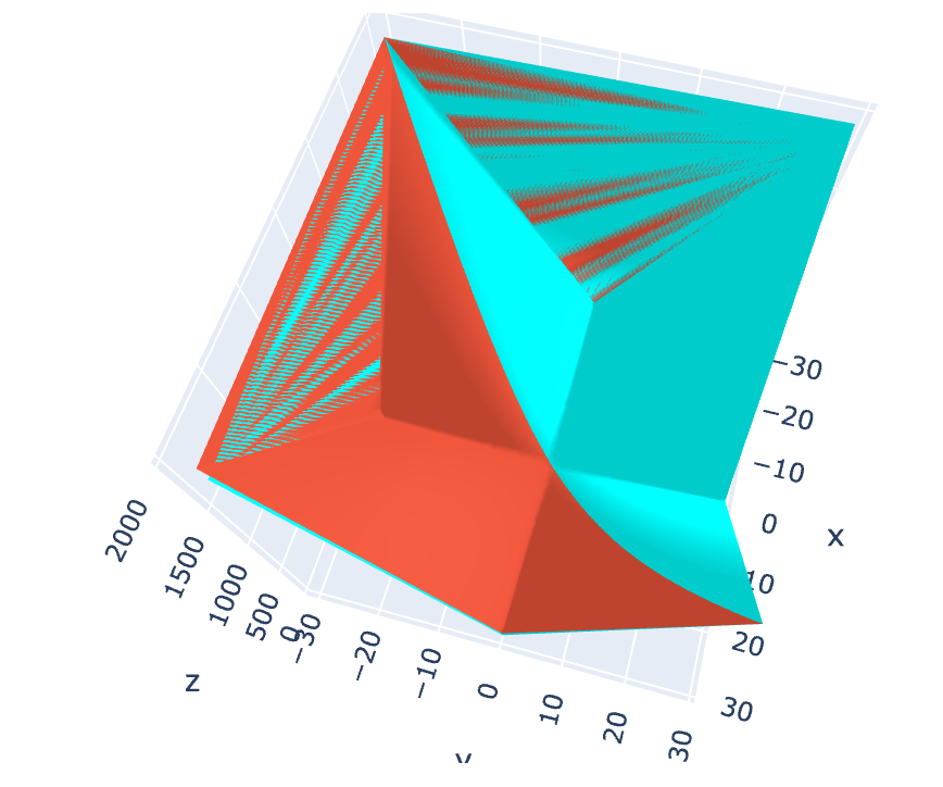
Graphing the same function using XNOR and XOR on a 3-dimensional plane does however produces interesting and beautiful results:

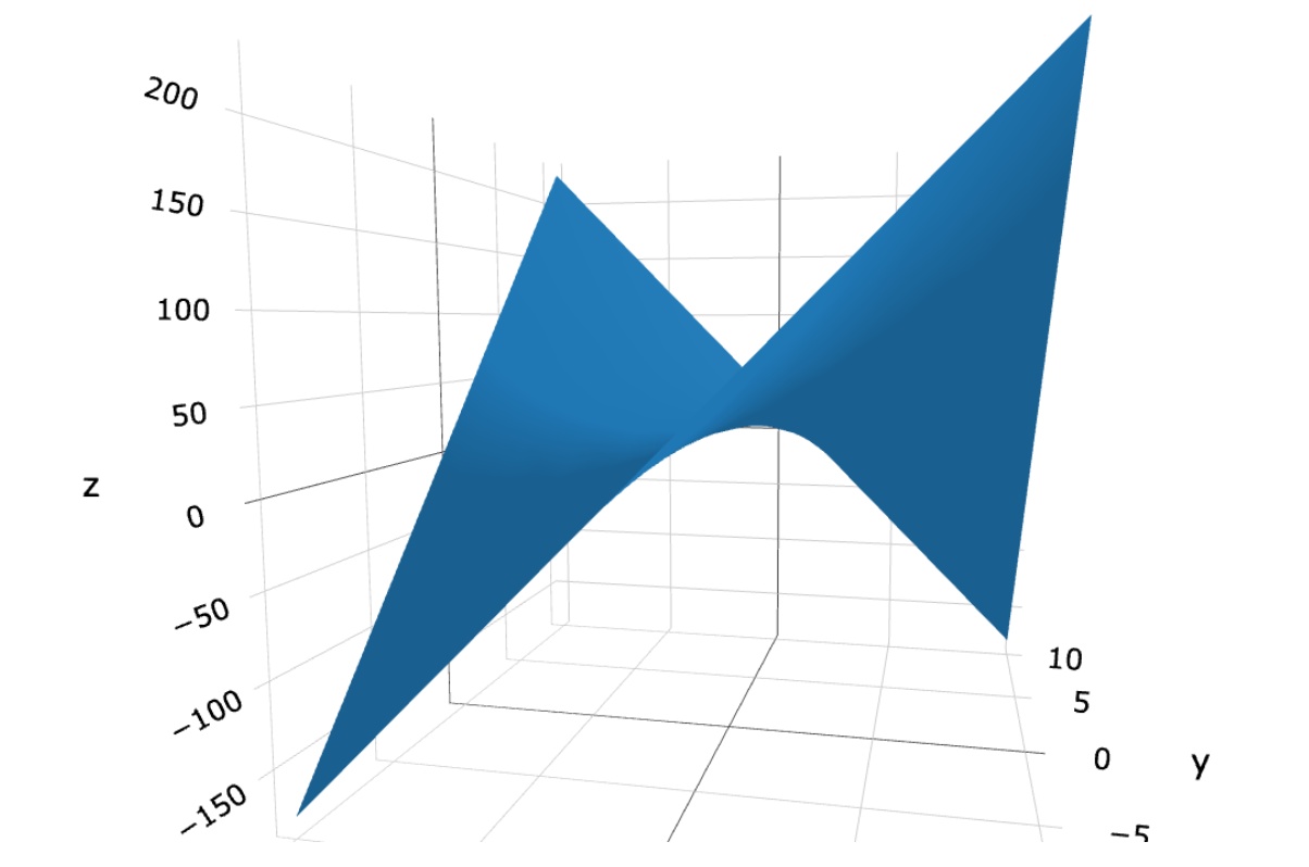
What this reveals is that the simple quadratic curve is a cross-section of this hyperbolic curve in Complex Space and not the cross-section of the yellow and green sheet our graphing program generated. This is a lot of information for a simple quadratic formula.

Plotting Domains

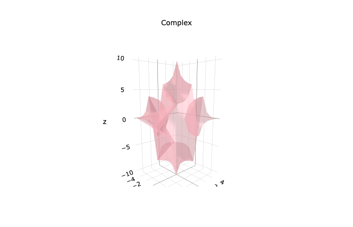
Now that we have our new rules for Logic Gate Algebra or Order 2, so called because it deals with two coordinates, we can begin plotting some functions. To start with I plotted results of all functions for (x!∆+y∆)(x1∆+y∆) over a finite field to produce:

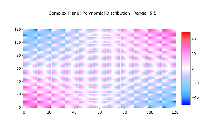
We can increase or decrease the range and increase the step value to produce many such graphs. Interestingly, they all exhibit the same properties at every scale, much like how magnetic fields exhibit the same properties no matter if they are produced by a single atom or a whole storm of atoms nested in a magnetised block of metal.

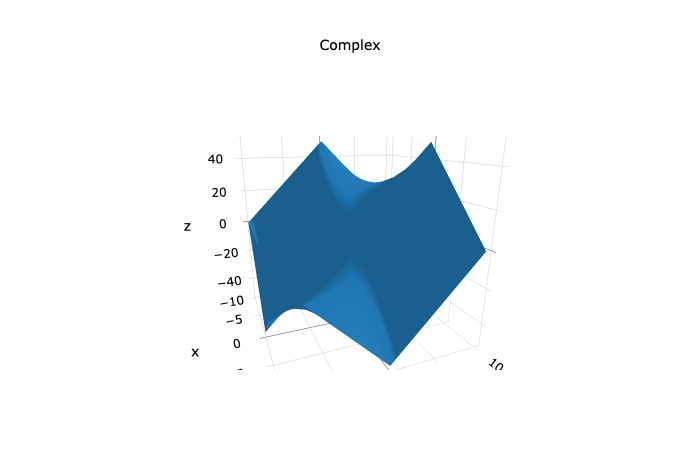
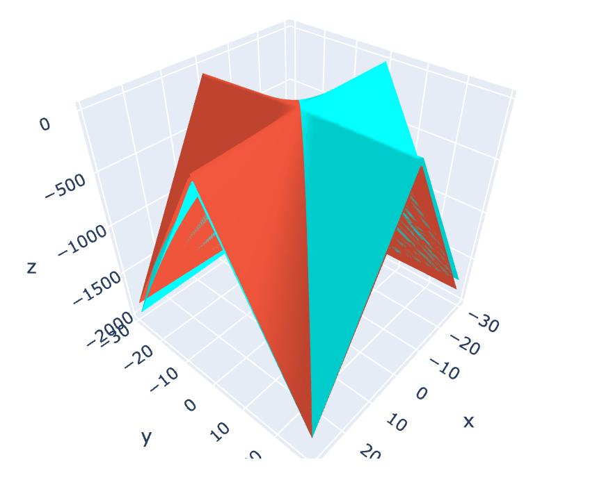
Graphing a single function is more revealing. In this case it is the function from earlier: 2(!∆+3)(!∆+4);

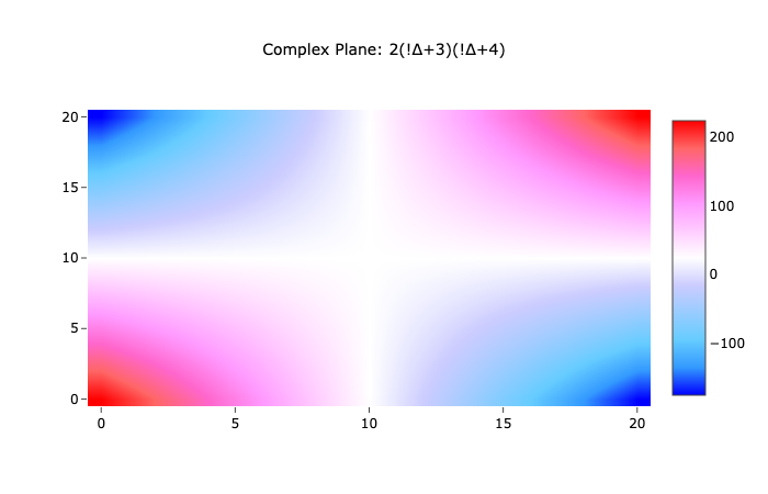
With this much simpler plot it is easy to see that what we are graphing here is simply the parabolic curve from earlier.

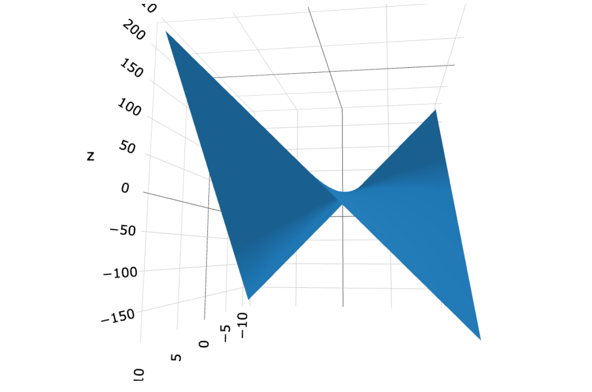
Figure 2: 2(!∆+3)(!∆+4) hyperbolic quadratic

So this, as we know is the general shape of polynomial multiplication in the Logical Gate Space. But what about polynomial division algebras?

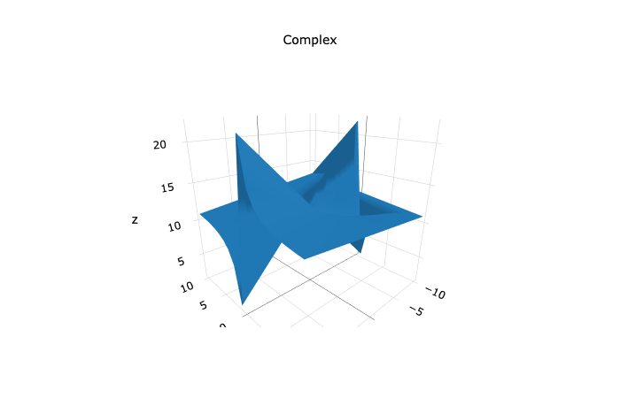
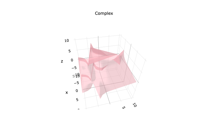
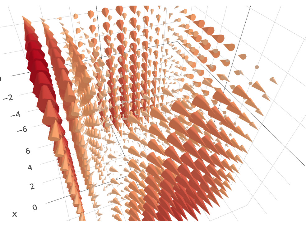
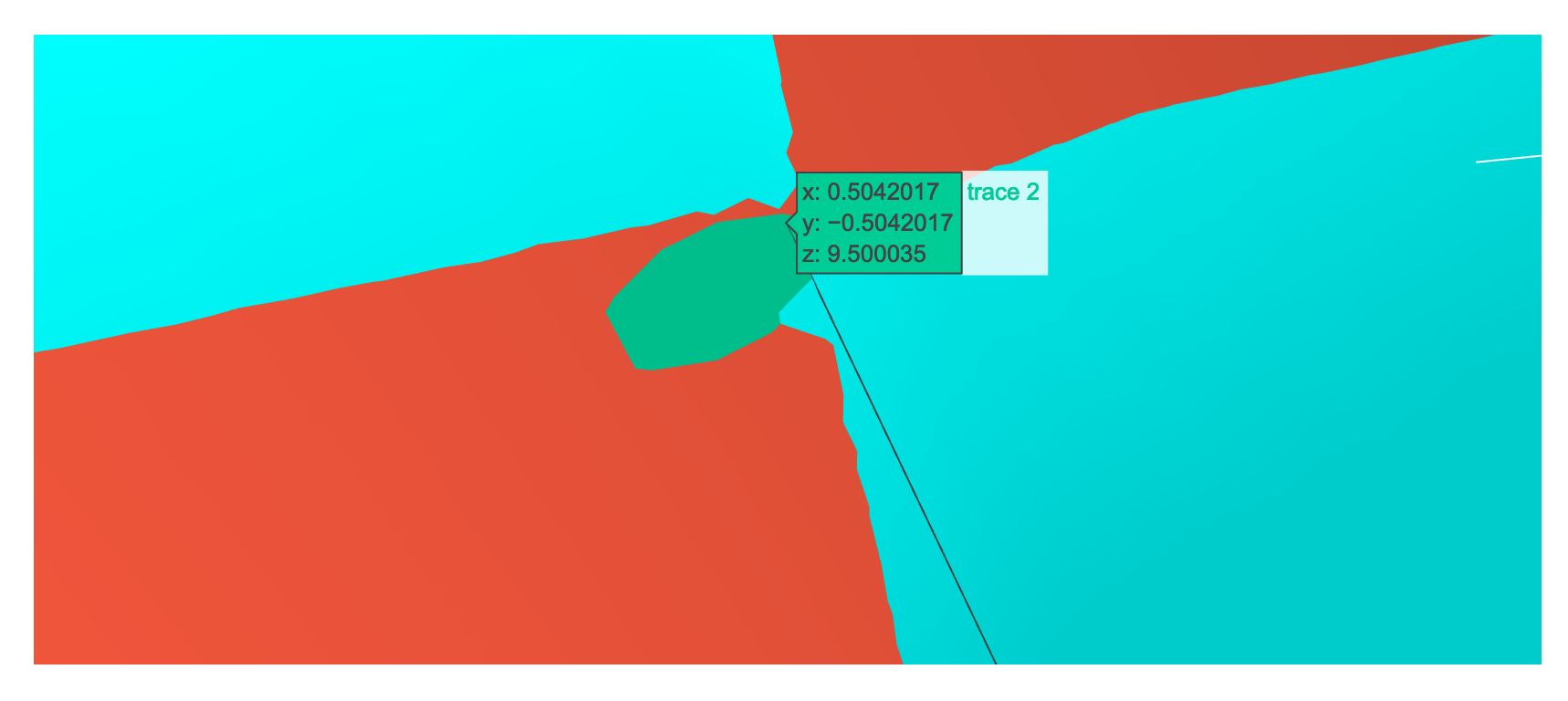
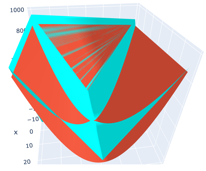
Figure 3: 2(!∆+3)/(!∆+4) hyperbolic Division Quadratic

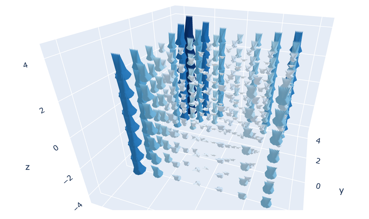
Here we have (x!∆+3∆)/(y!∆+4∆), which produces this unusual ‘saw-toothed’ graph. The results for all functions of this kind, over a particular finite range can be plotted in 3D and reveal the same structure. This is interesting and shows that these functions are somehow embedded in themselves. I’ve used a less opaque surface here to make the resulting structure more apparent.

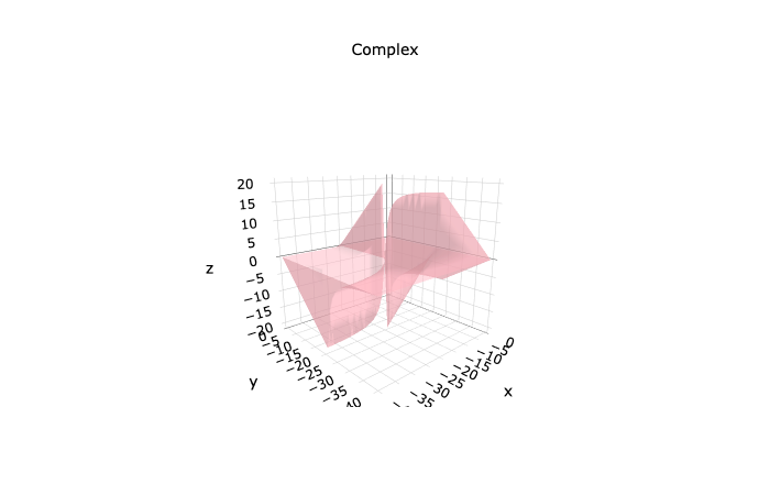
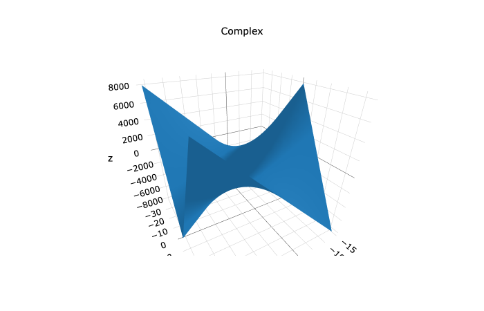
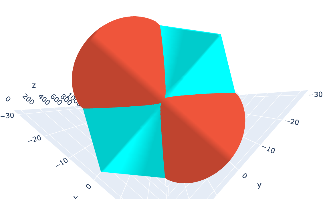
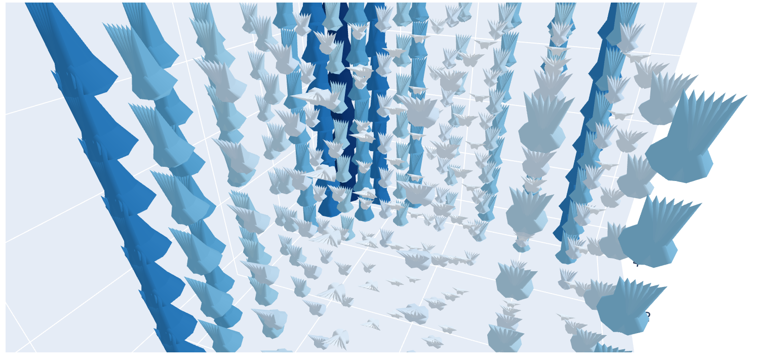
Figure 4: Polynomial Division

The major difference between more general division functions like these and the previous multiplication functions is revealed when the range of the field is increased. These functions appear to show repeat patterns extending out across the plane, whereas the other one just stays in place and increases to infinity. Below, we have one section of the above function (left) and then an extended version (right). The graph on the left is embedded in the graph on the right, although it helps to be able to rotate the two graphs to compare the shapes to see exactly where it is embedded. The other peaks and troughs hint that this structure repeats outside the limits of the field, but exactly how and in what way is not yet known, as it requires a large amount of processing power to generate such graphs.

Figure 5: Embedded and Extended graphs

3-Dimensional Cubic functions are enabled by (x+y)^2, which was unexpected because the function is squared rather than cubed. The Plotly graphing library used to generate this has a bug in it that glues some of the faces together with unwanted polygons. I’ve had to angle this graph so they remain hidden. Unfortunately this may not be the best angle to view the cubic properties from, but it should give the reader some idea.

On the plus side, there is a way of altering the parameter alphahull, which when set to zero joins up all the faces of this cubic function to reveal a cuboctahedron; an object with 6 square and eight triangular faces.

Figure 3: (x!∆+3)^3 hyperbolic Cubic

Graphing (x!∆+3)^3 results in the following hyperbolic cubic function. The alphahull = 0 of this graph equals a nicely skewed octahedron.

I don’t know if this means that there is a relationship between 3D cubic functions and platonic solids, but it is interesting to speculate about.

Plotting (∆, !∆, ∆)^2 gives you the familiar saddle graph:

Figure 8: Saddle Graph

For the most part, representations of the complex plane is done in two dimensional heat maps. But two extra real space dimensions can always be added to these spaces making them 4-dimensional in total.

It is impossible for the average human to visualise or imagine the fourth dimension, but there are ways and means around this. For instance, we could plot three of our values as real space coordinate values and allow the fourth to be some kind of vector coordinate, denoting direction or flow. This works quite well. Another method is simply move each of the four dimensions in and out of the three real space dimensions at a time, giving you a ‘slice’ or a window into what the entire function might actually look like. This is not very satisfactory, but for us mere 3-dimensional mortals, it is often the best that we can do.

Graphing the saddle plot from fig. 6 in vector coordinates gives the following results;

Figure 9: Saddle Graph using XNOR Vectors

Something like this might represent aspects of quantum field mechanics; like the flow of charges in an electrical field. If so, Logic Gate Algebra may provide students and mathematicians alike with a simple and logical method of graphing numerous different four-dimensional fields. If these fields can be shown to be analogous to particles and/or particle interactions in the real world, then there may actually be some validity to the idea that quantum particles exist as a confluence of dimensions, all with their different modes of multiplicative arithmetic, based on four bit binary numbers. And if not, then at least it might serve as a basic pedagogical tool to teach the principles of quantum mechanics to young students.

Pure Math in LGA

Using ‘i’ as an algebraic representation of √ -1  is a powerful tool for understanding the world. The stated reason for using this convention over some other one, is that we don’t have to invent new numbers. In short, it keeps things nice and simple. But, as we have seen, the result of using ‘i’ has led to the discovery, or invention, of the Quaternions, Octonions and Sedenions (to name but a few) and their associated Lie Groups and Clifford Algebras, so new number systems are a direct consequence, either way you look at it. Transformation of Quaternions into SU(2) are needed to create a Norm-Division Algebra. This has been tremendously useful in Quantum Physics and Relativity. But nobody could say that it is ‘simple’, quite the opposite in fact, it is among the most difficult maths any mathematician has to contend with.

So how does LGA compare with these other methods?

As we have seen, LGA works fine for when we are multiplying and dividing, but what about other areas of arithmetic? How does LGA deal with something simple like (a+b=c)? The answer is far more difficult than we would at first imagine. Let’s take a look at the rules for addition in XOR:

As we can see, these are identical to the multiplication rules of XOR. Now lets look the same rules in XNOR:

They are just the opposite. In light of this, we can do arithmetic at all stages across the divide of the XNOR and XOR dimensional axes or gateways. But how does this work with some simple real world examples? If we have the sum 4+6=10 (in XOR) and we exchange the operators, we get:

In XNOR, we get the complete inverse:

How does it work on the Complex Plane? For example, how does it deal with something like the Riemann Zeta Function? The Riemann Zeta function contains an infinite series of the kind:

Re(z) = 1/1^(a+bi) + 1/2^(a+bi) + 1/3^(a+bi) + 1/4^(a+bi) + 1/5^(a+bi)...

where ‘a’ and ‘b’ are Real numbered values and ‘i’ is of course the imaginary number. Working out the first three terms of the Riemann Zeta function in this fashion, results in;

1/1⁽²⁺³ⁱ⁾ + 1/2⁽²⁺³ⁱ⁾ + 1/3⁽²⁺³ⁱ⁾

(∆1 +(- !∆1)) + 1/(4 + (-6)) + 1/(6 +(-9)

∆: 0 + 1/-2 + 1/-3 !∆: 2 + (+1/10) + (+1/15) 

∆: -0.5 +(-0.333333…) 

! ∆: 2 -0.1 - 0.0666666… 

∆: -0.833333… !∆: 1.833333… 

∆: - 0.833333… + 1.833333… = 1

!∆: - 0.833333… + (+ 1.833333…) = 2.666666… 

Therefore the result in coordinates is; (1, 2.666666). This is another level of LGA and is fully stocked for all arithmetic, not just multiplication and division. As such this will be labelled LGA-1, whereas our previous system will be labelled as LGA-2. Arithmetic in LGA-1 is admittedly confusing. More work needs to be done on which operators pertain to XOR and which to XNOR and how they interact, otherwise the calculations will result in inconsistent results. For a more in depth analysis of how LGA-1 interacts with the Riemann Zeta function take a look at insert link here.

Other series that are useful to do real mathematics include the Taylor Expansion for trigonometric functions for Sin, Cos and the Exponential function. By applying the same rules of arithmetic to these functions, as above, we see that they equate to Sin(x) = —y, Cos(x) = y and the exponential function exp(x) = y-x.

16-Dimensional Spaces

The LGA are arranged from ‘0000’ to ‘1111’ and ascribed letters ‘A’ through ‘P’.

Here 0 = ‘+’ and 1 = ‘—’. Notice that ‘G’ is equivalent to XOR, ‘J’ with XNOR. There are other logic gates here, for example, including; ‘I’, ‘B’, and ‘O’, which correspond to AND, NOR and NAND, respectively.

If we can think of these 16 systems as distinct rules for addition in multi-dimensional space, then we notice some interesting properties. For instance, no matter the operator in ‘A’ the answer is always a positive. The opposite is true for ‘P’. In many of these spaces, like ‘C’, ‘D’, ‘K’ and ‘L’, a positive number by a negative number yields different results depending on how they are multiplied together. For instance:

3C*-3C=-9

-3C*3C=9

This means that they are non-commutative in this respect. But in other respects, when the operators are the same, ‘C’ is commutative. I will refer to these groups, as ‘super-commutative’, from now on.

Hyperbolic Curves

One of the most famous demonstrations of the imaginary roots of a quadratic equation comes in the form of x²+1 = 0. Ordinarily, we think of this function as having no factors i.e. it cannot be written as a polynomial. However, if we rewrite this equation in XNOR and XOR, we see that we can generate a polynomial:

(∆!x + 1∆)(-∆!x + 1∆)

Plotting this gives us the usual hyperbolic polynomial curve that we have seen before. But what about other equations? Are there other equations that are considered to be completely factorised, which can be factorised further with this method? I don’t know, but we can look at other equations that are close to being factorised, like;

2x² + 2x + 10 = 0

If we pull the common factor out, we get:

2(x² + x + 5) = 0

If we make use of the 16-dimensional spaces (shown above) we can rewrite the original equation as:

(1A - xA)(-5I + xI)

where ‘A’ and ‘I’ are LGA spaces: ‘0000’ and ‘1000’ or AND. But how do we determine, which spaces we are to use?

The method I employed for this makes use of matrixes, cartesian products and set theory to narrow down the likely candidates. Once we have the candidates, we can start applying them to the quadratic matrixes to see if they satisfy the result. But there is a much simpler method, which we will also look at in this section, using matrices, which are not unlike the Pauli matrices.

The result (1A - xA)(-5I + xI) can then be plotted. But before we do that. Let’s take a look at usually meant by a hyperbolic curve in algebra using the same coefficients as in the earlier examples:

Figure 10: What is ordinarily thought of as a Hyperbolic Quadratic.

As we can see this is just a saddle graph. Whereas graphing (1A - xA)(-5I + xI) gives us what we have been calling a hyperbolic graph:

Figure 11: An actual Hyperbolic Quadratic made from Logic Gates.

We can plot them all together, to show that (1A - xA)(-5I + xI) produces a much better match for the curve than the saddle graph does:

Figure 13: Comparison of various related quadratic shapes.

Here the green surface is just (2x² + 2x + 10). Notice how it aligns with the aqua-coloured graph, whereas the red graph not so much. The roots of this expression are at (0.5, 2.1794) and (-0.5, -2.1794). These coordinates are located in the centre of the green patch below:

Figure 14: Roots of quadratic functions.

What about expressions without imaginary roots that are close to being factorised or completely factorised? Can these be graphed in higher dimensional space? The answer is ‘yes’. Let’s take 2x² + 4x + 2. It’s roots are x=-1. Taking out the common factor, we have:

x² + x + 1

If we were to make a matrix out of this, we get:

, which equals: x² + 2x + 1. So this is not right. In order to make it fit the function, we can apply logic gates ‘A’ and ‘P’ to the matrix, to get two new matrices.

We multiply the matrix on the left by 2, then multiply both matrices with our original matrix and sum the product to create:

This gives us our original expression: 2x² + 4x + 2. Now, all that is required is to divide by 2 and we have x² + x + 1, or:

(xA+A1)(-xA-1A) + (xA+P1)(-xP-1A)

Conceivably, a similar process could be applied to create any quadratic without imaginary roots. Once we have our expression, we can plot it over a range to produce a graph. Previously, these graphs included imaginary numbers and were, in some sense, considered 4-dimensional. Our newest expression was created using the 3 real-space dimensions and two other imaginary dimensions ‘A’ and ‘P’. As a result, we may consider the totality of the output to be 5-dimensional. Although, this is debatable as ‘A’ and ‘P’ are constructed entirely out of pluses and minuses respectively, which when summed produces ‘G’ or XOR. If this is the case, then ‘i’ doesn’t represent a 4-dimensional axis, merely another way of looking at our 3-dimensional axes.

Figure 15: (xA+A1)(-xA-1A) + (xA+P1)(-xP-1A) and its inverse (meaning multiplied by minus 1)

When several of these dimensions are graphed simultaneously, we see the shapes above. The figure on the right is the inverted version of the one on the left. The line bisecting the graph on the left is our quadratic curve.

This is further demonstrated in the graphs below, where the red trace equals (x² + x + 1) and the aqua-coloured trace equals (xA+A1)(-xA-1A) + (xA+P1)(-xP+1A):

Figure 16: (xA+A1)(-xA-1A) + (xA+P1)(-xP-1A) compared with the garden variety (x² + x + 1).

We can attempt to plot our simple 4D parabolic equation in a vector space to get a better understanding of what it might look like in higher-dimensions. I say ‘attempt’, because it is clear that vectors are not the right tool for this job. A better tool would simply show how much our original coordinates ‘x’, ‘y’ and ‘z’ (which are simply the starting coordinates of our system) are displaced by our LGA new coordinates.

Since a simply and obvious transformation like this is not permitted in vector graphs, I decided to play around with it and generate a 5 or 6 dimensional graph illustrating some kind of field based on our quadratic formula.

Figure 17 and 18: (xA+A1)(-xA-1A) + (xA+P1)(-xP-1A) as a 4-dimensional system.

The graph is simply four spatial coordinates, with the ‘y’ coordinate repeated in the ‘v’ coordinate and the quadratic; (xA+A1)(-xA-1A) + (xA+P1)(-xP+1A). The result is interesting, because it shows that each point in the vector space has between 2 and 7 vector cones. All electro-magnetic fields fluctuate slightly (by about the mass of a photon). This method appears to produce such a fluctuation as a matter of course, without the need for any extra parameters.

Related Research

About half-way through writing this document, I thought it would be a good idea to check who else was working in this area. A very similar idea was put forward by Martin A. Hays, who has conceived of six different number systems using +0, -0 and the shape of the Necker Cube to generate a new mathematical system. A consequence or extension of this system incorporates logic gates to derive a very similar understanding of √ -1 , as laid out in this document. The inspiration, application and execution of Hays’ and my own methods are very different, however.

Conclusions

Logic Gate Algebra produces a well-ordered, commutative, and associative algebra that doesn’t rely on complex conversions to Lie Groups or Clifford Algebras. It should be noted that one LGA space is not necessarily commutative with another, but this is seen as a strength of the system, rather than a weakness, and has many applications in numerous fields outside of LGA, such as Quantum Mechanics. For more on this, see: The Shape of a Photon, by Christopher O’Neill.