Heisenberg Uncertainty Principle and DGO

Christopher O’Neill

BAEC, Civic Centre, Main Street, Bray, Co. Wicklow

Abstract

The principles of the Dimensional Gate Operators (DGO) can be applied to the models of the Heisenberg Uncertainty Principle acting on a sub-atomic wave packet. DGO replaces the algebraic notation of imaginary and complex numbers with a more accurate real numbered value, which allows us to see the results of equations and experiments, without the obfuscation of abstract terms. This provides us with a more complete understanding of the principles of Quantum Mechanics and which is more in line with both theoretical descriptions and experimental results. A liberal use of graphs is employed to make the results of this method even more apparent.

Uncertainty

There are various reasons why complex numbers are used in Quantum Mechanics. One of the key reasons is that they are seen explicitly in the Schrödinger Equation. The Schrödinger Equation models the wave form of a particle () in a box with infinitely high walls that prevent the possibility of the particle escaping.  A consequence of this equation is that the energy of the particle becomes quantised, as a result of the nodes of the wave function i.e. where  = 0.  The probability of the particle appearing at the node is less than zero. The particle is most likely to be found midway between two nodes.

Elsewhere, imaginary numbers are employed to explain a particle’s momentum and position as two different and interlinked properties. Knowing the momentum of a particle exactly, results in its position being everywhere at once and vice versa. To avoid running into these infinities, we can only ever know these two properties of the wave function approximately. This level of uncertainty is a consequence of the Schrödinger Equation and the Heisenberg Uncertainty Principle. It emerges because the probabilities of the two states are proportional to one another and must equal 1. Complex numbers also appear in the equations used to derive these probabilities, so they are a reoccurring feature throughout all levels of QM. The infinities of the Heisenberg Uncertainty Principle can be demonstrated by finding the absolute value of these complex numbers:

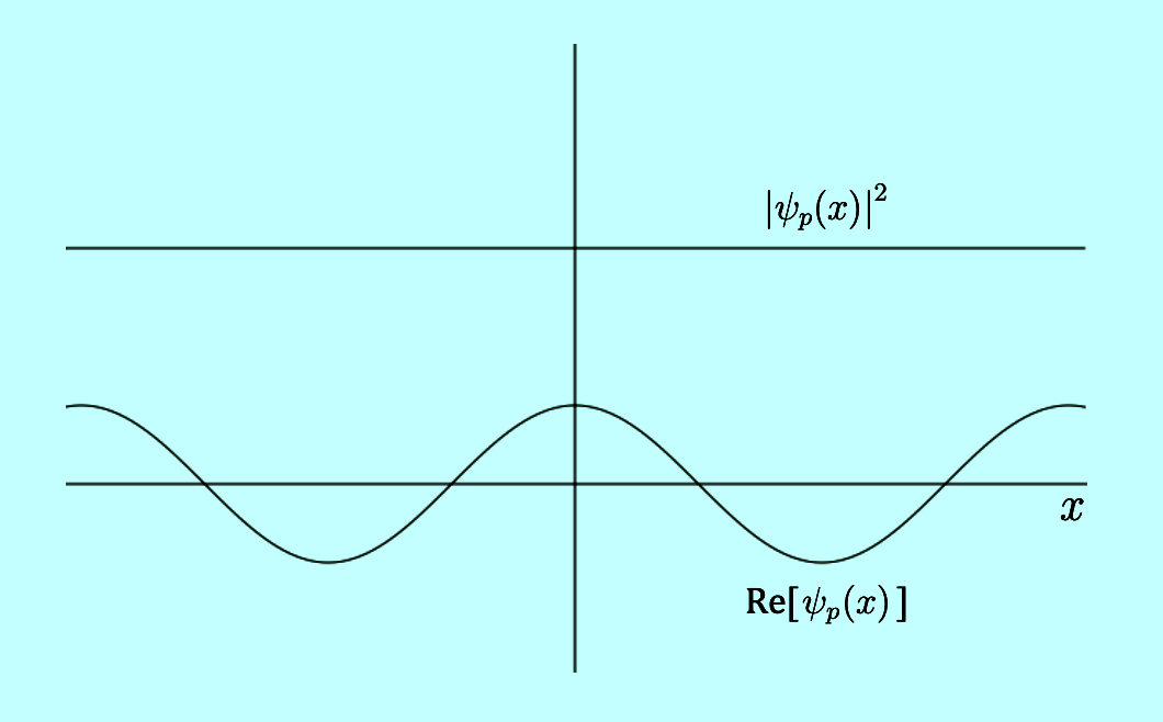
Fig 1: The traditional method of graphing Re[_p(x)] and its absolute square value.

The source of Fig 1 is taken from a paper by Ricardo Karam entitled ‘Why are complex numbers needed in quantum mechanics?”

Here, the absolute square of the wave function exhibits a flatline, which  indicates that the wave function is oscillating at infinite values. Notice, however that it is artificially raised above the zero-line of the x-axis, by some unspecified amount, in this diagram. Therefore it has no nodes. The particle can be found on at every point on this line. But is this the only solution to this problem? And how do we know that it is correct, seeing as how we can’t test it?

DGO Method

Using the logic gate arithmetic of DGO (in particular XNOR (!∆) and XOR (∆)), we achieve similar results. This is because XOR and XNOR are non-commutative, !∆.∆ + ∆.!∆ = 0. When we have two systems, they can be multiplied together. But when we have two different multiplication systems, each system must be cross multiplied, and the results summed together.

The wave packet of a sub-atomic particle can be modelled in the following way:

2 * exp(-0.25*x²) * cos(10*x)

Graphing this produces the familiar position-state wave-packet:

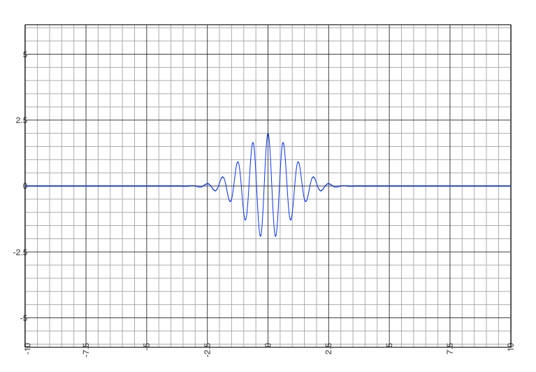
Fig 2: The wave packet of a sub-atomic particle showing the position-state of the particle, in this case a photon. As per the Schrödinger Equation, the energy of the photon is quantised, or bundled together in discrete packets, between where the wave function crosses the x-axis.

To calculate the same wave in XNOR, which is equivalent to the momentum of said particle, we simply switch the signs:

-2 * exp(-0.25*-x²) * cos((10*x)*-1)

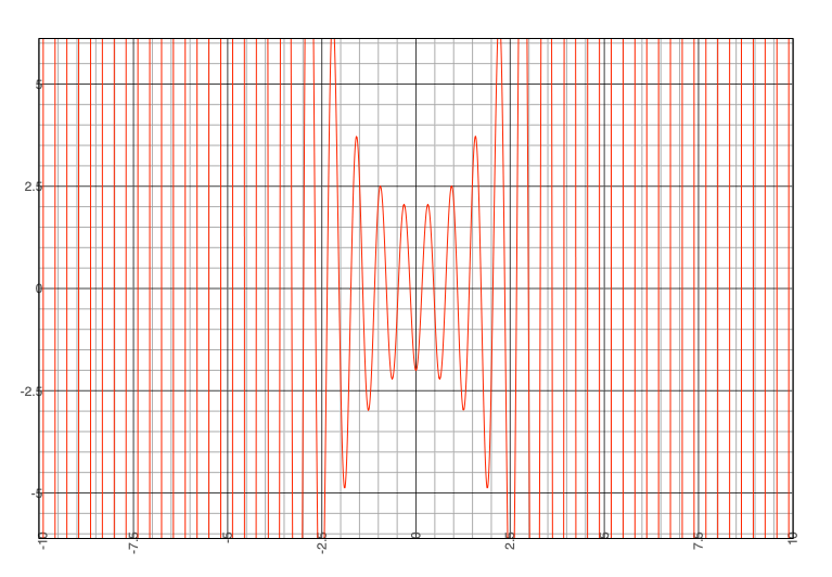
Fig 3: The momentum-state of the photon seen in Fig 2.

The result, as you might expect, is the complete inverse of what we see in Fig 2. Notice how, outside of a certain range, the wave function goes to infinity, or is otherwise undefined. In XNOR space, this value is equivalent to our XOR zero. The momentum can only be properly read (inversely) when the numbers come down in number to the point at which they can be registered. This provides an interesting insight, as to how physics works in the XNOR dimension, at least from the perspective of XOR.

The next step is to multiply our XNORed equation with our original equation:

∆(2 * exp(-0.25*x²) * cos(10*x)) * !∆(2 * exp(-0.25*x²) * cos(10*x))

This produces the green cosine wave in the graph below:

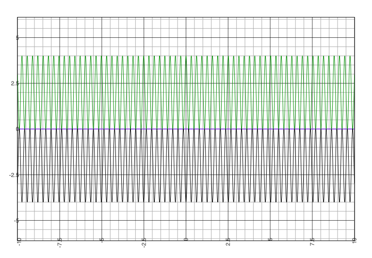
Fig 4

The black cosine wave is the result of multiplying the terms the other way around. Recall that we said that DGOs are anti-commutative:

!∆(2 * exp(-0.25*x²) * cos(10*x)) * ∆(2 * exp(-0.25*x²) * cos(10*x))

The purple line represents the sum of these two anti-commutative equations and is equivalent to our infinite result when either the position or momentum of our particle is known with utmost or absolute certainty.

Notice both cosine waves touch the x-axis at the same point along the x-axis, before eradicating themselves completely. This explains why a simple cosine or sine wave can be so effective at modelling certain aspects of quantum physics, because from one perspective that is what they are.

Asides from the new perspective that DGO gives us of the momentum-state in XNOR, it also provides us with several key steps that were missing from our earlier model. According to DGO, before the wave function is measured and collapses into infinity, it undergoes two radical state changes, characterised by the long cosine wave functions.

When all five equations are plotted together we see an aesthetic and symmetric pattern emerge.

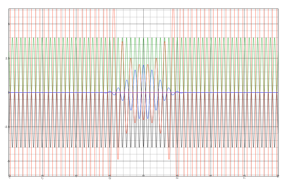
Fig 5: All five equations plotted at the same time.

All of these waves in Fig. 5 exist simultaneously depending on our measurement apparatus. The black and green cosine waves are intermediate stages between the infinite result of the HUP. But if so, why have they never been detected before? Perhaps they only exist for a very short period of time, or perhaps they are simply the underlying function and therefore never observed. But, I think we do have good evidence for their existence and for the accuracy of this model, as given by the Schrödinger equation and by experiment.

Notice how the green wave is twice as high as the position-state value (blue). This is just as we saw in Fig. 1. But there is a clear difference. Rather than a constant value across all points in space, they show an infinite series of discrete values across an infinite plane. This, then, is not our infinite wave, it must be something else.

The purple line is what occurs when both the momentum-state and the position-state are added together. This results in a zero or null value, which means that the particle is nowhere in space. Or said another way, this wave function is comprised completely of nodes.

Remember that from an XNOR perspective infinity was equal to zero. Therefore, it stands to reason that a zero result in XNOR equals to infinity. This implies that our particle, which now has either infinite position or infinite momentum also has infinite energy, which makes sense and relates to the fact that energy and time are also bound together in the HUP. Furthermore, this means that the particle could in theory escape our infinite box.

Conclusion

In conclusion, DGO offers a better understanding of the inter-relationship between the momentum-state and position-state wave function, than does the current model.